

Evidence for a Late Cainozoic Flood/post-Flood Boundary
Abstract
The Flood/post-Flood boundary in the geologic column can be determined by investigating geophysical evidence in light of Scripture’s record of the Flood. The following evidences are investigated:
(1) global sediment and post-Flood erosion,
(2) volcanism and climatic impact,
(3) changes in the global sea level,
(4) formation of the mountains of Ararat, and
(5) the formation of fossil fuels.
The evidences suggest that the Flood/post-Flood boundary is very late in the Cainozoic and most likely in the Pleistocene.
Originally published in CEN Tech. J., 10, no. 1 (1996): 128–167.
Introduction
Several years ago I realized that placement of the Flood/post-Flood boundary was crucial to understanding Earth’s geologic history, so I set out to find evidence for its proper placement. When beginning this research, I was slightly biased toward placing the Flood/post-Flood boundary near the Cretaceous/Tertiary boundary. This bias came from private discussions with creation researchers and reading creation research suggesting this location. It was only after collecting most of the data presented herein that I became convinced that the boundary was much later in the geologic record.
The location of the Flood/post-Flood boundary in the geologic record is important because of its tremendous impact on interpreting events during and after the Flood. The boundary is the key to understanding Earth’s geologic history, as its determination sets limits on Flood/post-Flood erosion, sedimentation, volcanism, continental sprint and drift, tectonic activity, sea level changes, etc. The location of the boundary simultaneously sets limits on pre-Flood and post-Flood biologic diversity and biologic change, and climatic variations in post-Flood times. Placement of the boundary in the early to middle portions of the geologic column implies tremendous post-Flood catastrophism, explosive biological change,1 and huge post-Flood climatic variations. A late placement of the boundary implies a more violent Flood, little post-Flood catastrophism, little biological change, and limited climatic change beyond a single post-Flood Ice Age. A comprehensive creation model cannot be developed separate from a definitive placement of the Flood/post-Flood boundary.
The end of the Flood, or more precisely the end of the year of the Flood, is the day that Noah and the animals left the Ark. This day corresponds to a geologic boundary or physical surface which is the Flood/post-Flood boundary. Identification of the boundary can be on a local, regional, or global basis, depending on the evidence and nature of the stratigraphic record. The focus of this paper is identification of the boundary on a global basis and in regions cited in Scripture.
Acceptance of a number of observations or generalisations about Earth’s geology are necessary to discuss the location of the Flood/post-Flood boundary on a global level. They are:–
- (1) the geologic column represents the sequential order of strata found throughout the Earth (this does not imply that most or all sections of the column need be present at any location),
- (2) the order of strata corresponds to the sequence of deposition, with limited exceptions (overthrusts, redeposited strata, mistaken strata identification, etc.), and
- (3) strata of the same geologic age (era, period and epoch) are penecontemporaneous (approximately contemporaneous).
A consequence of these observations is that the radioisotope ages assigned to strata, as biased or guided by stratigraphic considerations, are informative relative time markers though inaccurate in terms of real time. Some creationists might differ with these generalisations; I find them representative of the Earth’s surface and consistent with most creationists’ observations.
Agreement on one additional geologic point is required for discussing the location of the Flood/post-Flood boundary, namely, the stratigraphic location of the pre-Flood/Flood boundary. To my knowledge all creation researchers agree that the pre-Flood/Flood boundary is at or below the beginning of the Phanerozoic (that is, the Precambrian/ Cambrian boundary). Although this is an area needing more research, the agreement is sufficient for the present discussion.
An outline of the Genesis account of the Flood is illustrated in Figure 1. Important dates to remember are the 150th, 314th, and 371st days. Scripture indicates (Genesis 7:11, 24 and 8:1–5) that on the 150th day of the Flood (1) the Ark came to rest in the mountains of Ararat, and (2) the waters began to decrease off the face of the Earth. On the 314th day, Noah observed that the ‘face of the ground was dry’ (Genesis 8:13–14). On the 371st day, Noah’s family and all the animals left the Ark (Genesis 7:11 and 8:14–19). These three dates are significant events during the year of the Flood and place severe constraints on the Flood/post-Flood boundary.
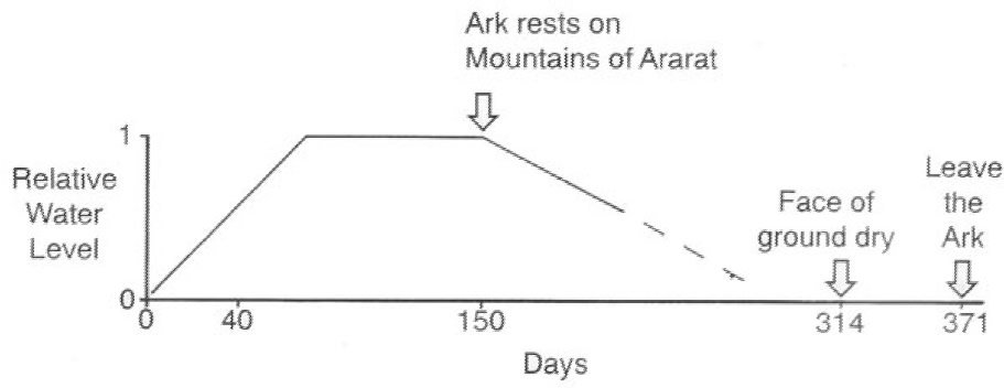
Figure 1. Simplified outline of the year of the Flood.
For modelling purposes, where necessary in the following discussions, the Flood is dated at about 4,500 years ago. The basis for this is as follows:
- (1) It is reasonable, if not appropriate, to take the genealogies of Genesis 5–11 as accurate and complete;2
- (2) The genealogies of Genesis place 1,656 years between Creation and the Flood; and
- (3) a straightforward reading of genealogies in Scripture indicates the Creation of the world occurred around 6,000 years ago.
This places the Flood at about 4,344 years ago; rounding to 4,500 years for simplicity.
A few creationists have suggested that the Flood occurred from 7,0003 to over 12,0004 years ago. This places the date of Creation even further back in time. I do not accept these suggestions because they
- (1) significantly harm the biblical chronology by introducing thousands of years into the genealogies of Genesis,
- (2) are based on questionable dating methods or presumed geophysical process rates, and/or
- (3) rely on the less accurate Septuagint.
Some have suggested that there was a significant time interval between the end of the Flood and the beginning of the Ice Age. This might lengthen the duration of the elevated post-Flood precipitation which includes the Ice Age. The potential for this interval, possible mechanisms, and its significance on the quantitative analysis from the various evidences will be discussed in the final section of this paper.
Prior Work
The stratigraphic or geologic identification of the Flood/ post-Flood boundary has been the topic of discussion among creationists for some time. Creationists early this century, such as G. M. Price,5 B. C. Nelson,6 and A. M. Rehwinkel,7 did not place much significance in the geologic column and suggested that all but the most superficial deposits were Flood deposits. Earlier creationists had similar views.8
In the last few decades, a number of creationists have acknowledged some value to the geologic column9,10,11,12,13 and some place the boundary deeper in the geologic column. Woodmorappe,14 Northrup,15,16,17,18,19 Scheven,20 and Robinson21 have placed the Flood/post-Flood boundary near the end of the Palaeozoic. Previously Austin, under the pen-name of S. E. Nevins, placed the boundary near the end of the Palaeozoic.22,23,24 Recently Austin,25 Wise26 and others,27 have placed the boundary at the end of the Mesozoic. Others, such as Whitcomb and Morris,28,29 and Coffin and Brown,30 have placed the boundary very late in the Cainozoic. The different placement of the boundary has resulted from a focus on different evidences, varying interpretations of evidence, and/or bias from different Flood-model paradigms.
Many different layers of the geologic column were exposed at the end of the Flood. The Flood/post-Flood boundary could therefore have tremendous local and regional variations. Locally the boundary could be interpreted as anywhere from the Cambrian to much higher in the geologic column. However, stating in a local context that the boundary appears in a particular geologic era, period, or epoch often conveys a global position of the boundary that may not have been intended. For this reason local or regional identification of the boundary needs to be tied to a global context. The global context is established if one accepts
- (1) the geologic column sequence as generally correct,
- (2) that strata of the same geologic age were, in general, deposited contemporaneously, and
- (3) the researcher does not limit his conclusion to a specific region.
In this global context, the Flood/post-Flood boundary is best identified by identifying the last geologic layer, epoch, or period that was deposited during the Flood.
Evidences used to geologically locate the boundary have usually included:
- (1) fossil content,
- (2) facies or presumed depositional environments,
- (3) the general change in fossil content with geologic strata, and/or
- (4) Flood-model paradigms.
Each of these methods have merit and limitations. In using these evidences many investigators implicitly assume that evidence for subaerial activity (geologic or biologic) is evidence for post-Flood activity.31,32,33 The reasoning for this assumption is as follows: evidence for subaerial activity indicates the area could not have been underwater, much less under the Flood waters, and hence subaerial activity must have been post-Flood. Although evidence for subaerial activity is consistent with post-Flood activity, it is not conclusive evidence of post-Flood activity. Uncritically accepting all evidence of subaerial activity is tantamount to denying the global Flood, because such evidence can be found through most of the geologic column.
There is room in the biblical account for subaerial activity in the early and late stages, and perhaps even in the middle of the Flood. The Flood waters did not instantly cover the Earth. There were forty days of rain before the Flood waters were deep enough to float the Ark (Genesis 7:17–18). No doubt there were areas higher in elevation than where the Ark was sitting; additional time would be required for these areas to be covered by the Flood waters. The ‘prevailing’ of waters for 150 days does not mean total covering all the time, because it was forty days before the Ark was floating and the waters had to ‘prevail exceedingly’ to cover all the high hills, and later the mountains (Genesis 7:19–20).
One should also not assume, a priori, that the waters increased and decreased in a monotonic manner over the entire surface of the Earth. While the waters prevailed on the Earth, for the first 150 days of the Flood, it is not certain that all areas were simultaneously covered by water.34 Some areas may have been repeatedly covered and uncovered by the Flood waters, while other areas may have been above water for weeks or months. God states his purpose for the Flood was to destroy man and all living creatures that had the breath of life in their nostrils and were living on dry land (Genesis 6:7 and 17; 7:21–23). God did not say water was to cover all areas simultaneously and continuously for 150 days.
God tells us in Genesis 7 and 8 that:
- (a) Flood waters began to decrease off the face of the Earth on the 150th day;
- (b) on the 314th day the face of the ground was dry; and
- (c) Noah did not leave the Ark until the 371st day.
Within the biblical description there is ample time for late Flood subaerial activity, more than 56 days but less than 220 days. In view of the Scriptural account, subaerial evidence should not be accepted as conclusive evidence for post-Flood activity.
Cited evidences of post-Flood subaerial activity include upright trees (assumed to be in the growth position), dinosaur nests, desert sands, unsorted volcanic ash and tuff, etc. One published claim35 that an upright tree grew in place was not supported by excavation of tree roots. Evidence presented did not eliminate the possibility that the tree was deposited upright by water as has been observed at Mt St Helens,36 and elsewhere over a century ago.37
Dinosaur nests are usually considered evidence for continued subaerial activity. However, there is important evidence that dinosaur nests did not remain on dry land long before they were buried catastrophically. The different nests in Montana have been described as eggs buried in mud inside a mudnest, and a ‘salad’ of baby dinosaur bones jumbled in three dimensions in green mudstone.38 One nest had been made ‘in the floodplain of a stream’ and Egg Mountain is described as ‘a peninsula or island in a lake’.39 Dinosaur eggs were found standing vertically in an unstable orientation, that is, on the small or pointed end.40 This orientation is characteristic of eggs submerged in muddy or mineral laden water, not a nest that remained on dry land.41 Dinosaur nests could date from the first 150 days of the Flood while waters were still rising.42
The Coconino Sandstone covers 518,000 km2 of the American south-west and averages 96 m thick. This massive deposit has routinely been interpreted as a desert with large wind-blown sand dunes. Recent investigations of animal trackways found in the Coconino Sandstone indicate the sand was water deposited.43 The character of the sand dunes are not like those produced by wind, but like dunes produced by underwater ‘sand waves’.44 Thus what was considered evidence for subaerial activity is now evidence for submarine activity.
‘Poor textural’ sorting of volcanic tuff and ash in the John Day Formation (north-eastern Oregon) has been interpreted as evidence of subaerial activity by one observer,45 while another sees evidence of reworking by water.46 In contrast to the subaerial interpretation, ‘the deposits of airfall tephra, unlike those of pyroclastic flows, are generally well bedded and well sorted.’47 However, at Mt St Helens an extensive 8 m thick stratified deposit, with thin laminae and cross-bedding, was formed in less than one day by a pyroclastic flow.48
Turbulent air or water flow produces less sorting than laminar flow.
‘Sorting (by wind) is most effective among ejecta of sand-sized and fine gravel-size, and least effective among bombs and lapilli (grain size >2 mm), on the one hand, and extremely fine ash, on the other. . . . Fine glass dust may float for long periods on fresh water, but tend to coagulate and settle rapidly in brackish water or in the sea. Fragments of pumice, especially if they are large can float for great distances and may sink more slowly than dense particles of smaller size. This is why pumice and ash deposits laid down in lakes and seas usually have reversely graded bedding.’49
Textural sorting of ejecta is highly dependent on the conditions and rate of deposition; it is not a clear indicator of subaerial or submarine deposits. Scientists still have a lot to learn about rapidly forming deposits.
Evidence listed by those advocating a late placement of the boundary include the absence of a worldwide unconformity, fossil formation (which requires rapid burial), merging of formations, and the absence of time breaks between strata.50 The local or regional nature of Cainozoic sediments and the change in fossil animal types are what some would predict from the receding Flood waters,51,52 while others believe this indicates a post-Flood environment.53
Published evidence for the Flood/post-Flood boundary has not been conclusive, and there is a wide divergence of opinion in interpreting the evidence. The purpose of this paper is to present more definitive evidence for the geologic location of the Flood/post-Flood boundary. To do so requires
- (a) making quantitative assessments of the geophysical activity associated with the placement of the boundary, and
- (b) tying the boundary directly to the Scriptural account.
The following evidences are investigated in this manner:
- (1) global sediment and post-Flood erosion,
- (2) volcanism and climatic impact,
- (3) changes in the global sea level,
- (4) formation of the mountains of Ararat, and
- (5) the formation of fossil fuels.
Each of these evidences places severe constraints on the Flood/post-Flood boundary and indicates the boundary is located late in the Cainozoic, and most likely in the Pleistocene.
Global Sediment and Post-Flood Erosion
Most of the continents and ocean floor are covered with sediment. Only a limited amount of sediment could have been moved or created by erosion since the Flood. One can make an estimate of where the Flood/post-Flood boundary is in the geologic column by comparing the maximum plausible amount of post-Flood sediment to the existing global sediment. To determine the location of the boundary in this manner the following information is required:
- (1) estimates of the mass and distribution of Earth’s sediment,
- (2) limits on the amount of post-Flood precipitation, and
- (3) limits on the amount of post-Flood sediment eroded and/or re-deposited.
Global Sedimentary Mass Estimates and Distribution
The amount of Phanerozoic sediment distributed in geologic sub-eras and periods is shown in Figure 2. The distribution is not uniform in radioisotope time or in geologic setting. The amount of sediment in the Tertiary is the largest of any sub-era or period, and that in the Quaternary is the smallest. The total amount of Phanerozoic sediment is estimated at 2.3 x 1024 g.
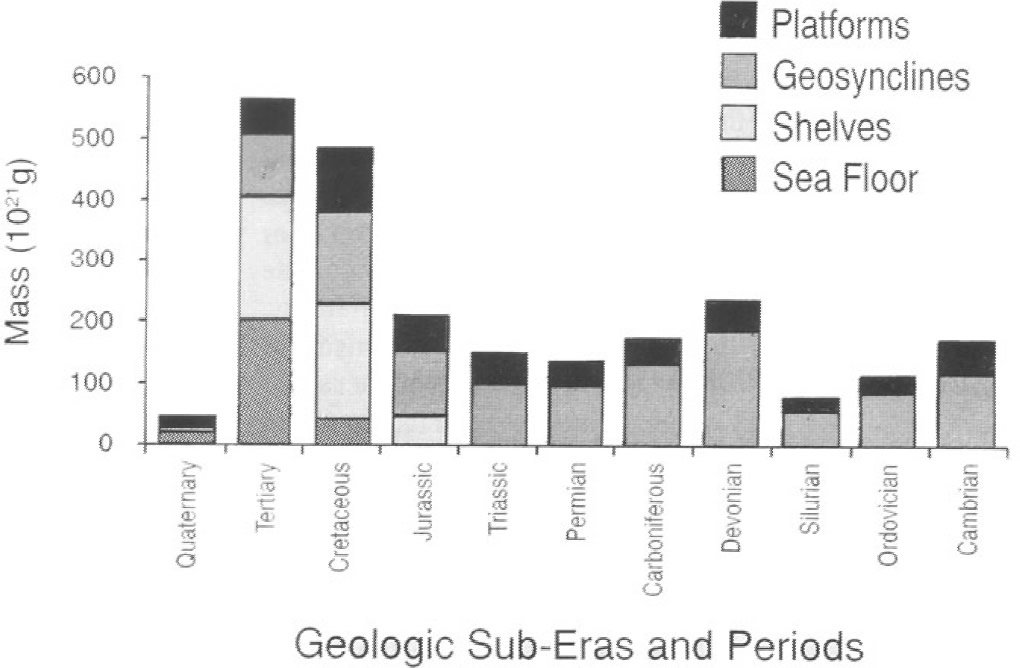
Figure 2.
The quantitative estimate of Phanerozoic sediment in Figure 2 is based on the work of Ronov et al.,54,55,56 Hay,57 and Hay et al.58 The data from Ronov et al. is the source for Phanerozoic sediment, excepting the Quaternary, on the continents and continental shelves and slopes. Their data provides the most comprehensive estimate of Phanerozoic sediment and is therefore used as the primary source of quantitative data. Hay provides the only global estimate of sediment for the Quaternary and is therefore used. The estimation of sea floor sediment from Hay et al. is used because it is more detailed than that of Ronov et al. and, perhaps, more accurate.
The data from Ronov et al. is based on a compilation of maps showing the lithologic associations, locations of crosssections, thickness of sediments, and isopach lines for all existing sediments. The maps are based on several decades of work by Ronov and others.59,60,61,62,63 The data has been the primary source for a number of studies of Earth’s sediment by various authors,64,65,66,67,68 as no other researchers have gone to as much work in quantitatively characterising the change in Earth’s sediment in geologic time. Ronov estimated a maximum error of 25 per cent for earlier estimates (to 1978) with the greatest uncertainty in older sediments.69 His total estimate of Earth’s sediment is comparable to the estimate of others.70,71
Though there has been legitimate criticism of Ronov’s earlier compilation,72 the data has been revised. In 1984 the Palaeozoic data (in the form of maps) was revised and expanded to include Antarctica.73 New sediment estimates for continental land, shelves and slopes, and the ocean floor must be in other maps, as published summaries include revised data for all the Phanerozoic, except the Quaternary. Rather than repeating the laborious detailed assessments of sediment volumes, the published summaries will be used.
A partial summary of the revised data, including ocean floor and continental shelf sediment estimates, was published in 1987.74 When compared to the 1978 summary (which was published in 1982),75 the revision shows an increase of 36.6 per cent in Phanerozoic sediments (including volcanics). About 33 per cent of this increase is from the sea floor and continental shelves and slopes. New sediment estimates are provided from the Late Jurassic to the end of the Pleistocene, and for volcanic rocks throughout the Phanerozoic. Unfortunately this 1987 summary focuses on the history of the Earth’s atmosphere and does not provide an updated estimate of non-volcanic sediments for the Palaeozoic through mid-Jurassic.
The 1987 summary also shows a reduction of 3.1 x 10²¹ g in the Tertiary continental sediments (non-volcanic), with major changes occurring in the Miocene and Pliocene. In the Mesozoic there is a reduction of 5.5 x 10²¹ g in continental sediments (non-volcanics), with the bulk of the change occurring in the Late Jurassic. Significant changes in the distribution of volcanics were also made; these are discussed in the section on volcanism.
Hay provides the only global estimate of total Quaternary sediment at about 43 x 1021 g.76 Hay divides the sediment into four major groups:–
- (1) ocean basins,
- (2) marginal seas,
- (3) continental shelves, and
- (4) continental sediments.
The most accurate estimates are for the ocean basins and for continental glacial sediment. Hay’s estimate for nonglacial continental shelf and land sediment is uncertain and is based on
- (1) a projection of Pliocene sedimentary rates, and
- (2) an assumption that Quaternary continental rates of clastic sedimentation increased proportionally to other estimated rates of Quaternary sedimentation.
Of Hay’s total Quaternary sediment, 11 x 1021 g is estimated as the total non-glacial continental sediment.
The sea floor estimates in Figure 2 are from Hay et al.77 Hay’s estimate is much more detailed than Ronov’s. The two estimates are about the same for the Jurassic. In the Cretaceous Hay’s estimate is 26 per cent less than Ronov’s and in the Tertiary it is 68 per cent greater than Ronov’s. Hay’s 1988 estimate for sea floor sediment is a significant 88 x 1021 g larger than Ronov’s. Even so it is comparable, although somewhat larger than other estimates.78,79,80 Hay’s 1994 estimate for Quaternary sea floor sediments increases the total sea floor sediment by 5.4 x 10²¹ g over his 1988 estimate.
The amounts shown in Figure 2 are existing sediments and include volcanics. There may have been much more sediment in each layer that was lost by reworking sediment (that is, eroding one layer to become a later geologic layer) or lost to the mantle by rapid plate subduction during the Flood. Some estimates of erosion indicate a repeated reworking of sediments on a massive scale.81,82 Massive reworking is indicated by the many large-scale unconformities throughout the geologic column. Although the amount of reworking during the Flood is difficult to estimate, there is validity to the concept. Erosion estimates, within the old earth paradigm, indicate that the original sediment in each period may be dramatically more than that shown in Figure 2, particularly in the lower geologic layers.
Not shown in Figure 2 are the Precambrian sediments. Ronov estimates the Upper Proterozoic has 266 x 1021 g of unmetamorphosed sediments and 234 x 1021 g of metamorphosed sediment.83 There is an additional 26 x 1021 g of volcanics in the unmetamorphosed sediment, bringing that total to 292 x 1021 g.84 Most of these sediments are generally thought to be pre-Flood and are therefore not included in Figure 2.
Post-Flood Precipitation and Runoff
The amount of post-Flood precipitation limits the volume of river water runoff from the continents and ultimately the amount of post-Flood erosion and sediment reworking. Precipitation estimates can be divided into two main time periods:
- (1) the time between the Flood and deglaciation, which is the time of the Ice Age, and
- (2) all time since deglaciation.
The Ice Age is the only time during which one may account for massive sedimentary deposits, since it lasts the entire time between the Flood and deglaciation. As a result the primary focus in estimating post-Flood precipitation and runoff will be on the Ice Age interval. Estimating the amount of precipitation and runoff during deglaciation and after the Ice Age is not essential, because quantitative estimates of sediment can be made from stratigraphic data.
The simplest model for post-Flood precipitation, that has an objective basis, comes from the Ice Age model of Oard. Oard has predicted a post-Flood increase in precipitation, above the present level, resulting from a warm post-Flood ocean.85 A sufficient mechanism to heat, and perhaps even overheat the oceans, has been identified by Baumgardner.86 Recently the model for a rapid post-Flood Ice Age proposed by Oard has been confirmed and expanded by Vardiman.87 Vardiman has found that the continental interiors cool to below freezing temperatures in less than 100 days after the Flood.
Oard has provided extreme estimates of the length of the Ice Age, that is, the time to reach glacial or Ice Age maximum, from 174 to 1,765 years, with a best estimate of 500 years.88 For the purposes of modelling and understanding the effects of Ice Age duration on precipitation, runoff, and erosion, both a 1,000 year and 500 year time to Ice Age maximum will be considered. In general, the effects of a 1,000 year Ice Age maximum will be discussed first.
Oard has estimated limits on the available continental precipitation required to cool a warm 30°C ocean to the present temperature. His estimate for the increase in precipitation over land is between 7.1 and 9.6 x 10²² g of water spread out over the duration of the Ice Age.89 This is an increase in the average annual precipitation over land by 7.1 to 9.6 x 10¹⁹ g/yr above our present 1.11 x 10²⁰ g/yr,90 assuming a 1,000 year Ice Age. This increase in precipitation is expected to fall north of 40 degrees North and south of 60 degrees South, with most of the precipitation falling in the northern hemisphere. These regions will be called 40+/60- regions for brevity.
All precipitation over land does not become river runoff. A significant amount of precipitation is evaporated. Today 55.6 per cent of the global land precipitation is evaporated before returning to the oceans via rivers and underground streams.91 Figure 3 shows the present distribution, by latitude, of surface area, precipitation, evaporation, and runoff for the land area of the Earth.92 During the Ice Age a significant amount of land precipitation was converted into lasting snow and ice. This reduced the water available for runoff. To estimate the average annual ice growth, the total ice mass at Ice Age maximum is needed.
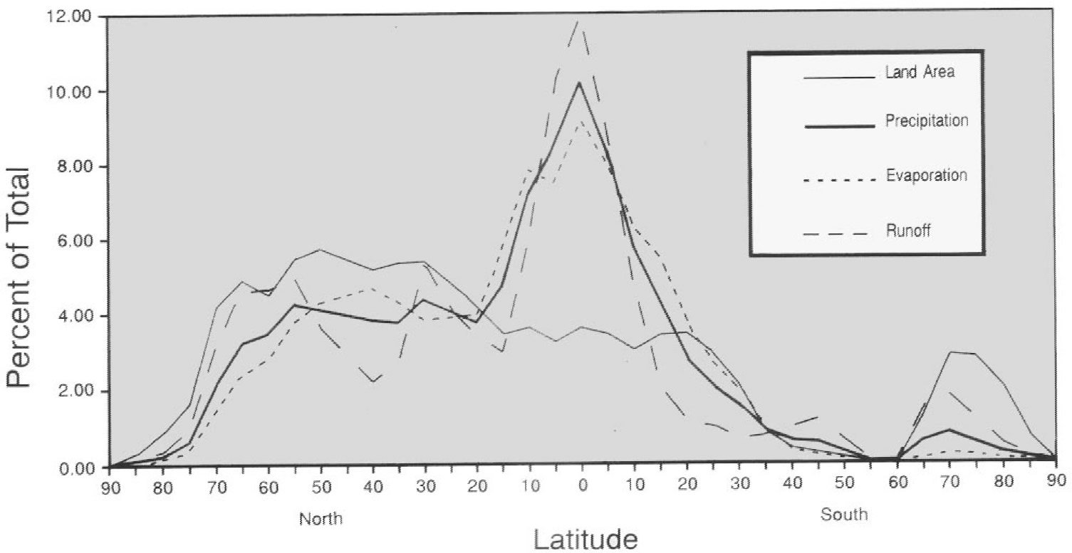
Figure 3. Present water balance for land.
Oard93 has proposed a sea level at -60 m during Ice Age maximum. He also noted that melting all of the present snow and ice would produce a +60 m increase in the sea level, if there were no isostatic adjustment. This suggests that at Ice Age maximum there was 4.33 x 10²² g of ice, calculating the change in ocean volume based on continental hypsography.94 This is 1.9 times the present global quantity of snow and ice. One can also estimate the total mass by using Oard’s estimated average maximum thickness for glaciers, and the known areas covered by glaciers. This gives a slightly smaller total mass of about 2.77 x 10²² g or 1.22 times the present global quantity of snow and ice. Evidence from sequence stratigraphy suggests that the Ice Age (Pleistocene) sea level was at about -85 m, ignoring isostatic adjustment and flexure of continental margins.95 If the sea was at -85 m, Ice Age maximum would have contained 5.26 x 10²² g of snow and ice, or 2.31 times the present global quantity of snow and ice.
To maximise the quantity of snow and ice present, 5.26 x 10²² g will be taken as the total at Ice Age maximum. The average annual snow and ice accumulation will be this quantity divided by the time to Ice Age maximum of 1,000 years. This average accumulation of snow and ice is then 5.26 x 10¹⁹ g/yr, which is about 25 per cent of the average Ice Age precipitation.
To place an upper limit on Ice Age precipitation and runoff, the following assumptions will be made in addition to those previously discussed:
- (1) The maximum additional precipitation predicted by Oard is added to the present precipitation only in the 40+/60- regions.
- (2) The annual precipitation in these regions is set proportional to the land areas, in 5° latitude increments.
- (3) Evaporation will be set equal to zero in all land areas to create a maximum runoff condition, even though it is very unrealistic.
- (4) All precipitation will become runoff, or snow and ice; runoff through underground aquifers is set equal to zero.
- (5) Significant volumes of snow and ice are restricted to the 40+/60- regions and are set proportional to the land areas, in 5° latitude increments, within these regions.
From these assumptions, one can calculate the resulting distribution of precipitation and runoff throughout the Earth. Baumgartner and Reichel have provided quantitative estimates of surface area, precipitation, evaporation, and runoff for land and separately the ocean, in 5 degree latitude increments.96 Adding Oard’s postulated maximum precipitation, setting land evaporation to zero, and adding snow and ice formation to the data of Baumgartner and Reichel provides estimates of post-Flood precipitation and runoff in 5 degree latitude increments.
When the calculated Ice Age precipitation is compared with present precipitation levels, the increases are by a factor of 3.3 for the 40–90N region, a factor of 1.0 for the 40N– 60S region, and a factor of 17.8 for the 60–90S region. The tremendous increase in the 60–90S region is because there is so little precipitation in today’s environment with a cold ocean; only Antarctica and a few small surrounding islands are in this region. Global annual precipitation increases by a factor of 1.9.
Ice Age runoff increases by similar factors. Major gains in runoff are due to the unrealistic elimination of evaporation. In the +40/–60 regions, runoff gains due to increased precipitation are reduced by losses in formation of enduring snow and ice. When the calculated Ice Age runoff is compared with present runoff levels, the increases are by a factor of 4.6 for the 40–90N region, a factor of 3.1 for the 40N–60S region, and a factor of 12.2 for the 60–90S region. The runoff in 60–90S appears large only because there is so little runoff in Antarctica today. The annual global runoff increases by a factor of 3.9.
To improve the model, evaporation over land at the present level will be assumed. The calculated annual global runoff is then smaller. The Ice Age runoff levels compared to the present runoff level increase by a smaller factor of 3.2 for the 40–90N region, a factor of 1.0 (that is, no change) for the 40N– 60S region, and a factor of 12.0 for the 60–90S region. The resulting annual global runoff increases by a factor of 2.1. Figure 4 shows the resulting Ice Age annual precipitation and runoff.
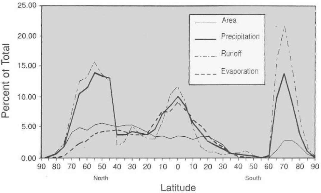
Figure 4. Distribution of precipitation, evaporation, and runoff estimated for the Ice Age.
Similar calculations were made for a 500-year long Ice Age. The results show higher precipitation and annual runoff as expected. Calculations were also performed for a reduced amount of ice based on Oard’s postulated maximum ice thickness in the northern and southern hemispheres (906 m and 1,673 m, respectively) and the areas covered by glaciers.97 The calculations show that runoff is increased if either, or both, the ice mass at Ice Age maximum or the time to Ice Age maximum is reduced. The precipitation and runoff calculations are summarized in Table 1. The total precipitation and runoff in a 1,000 year Ice Age is noticeably more than that for a 500 year Ice Age.
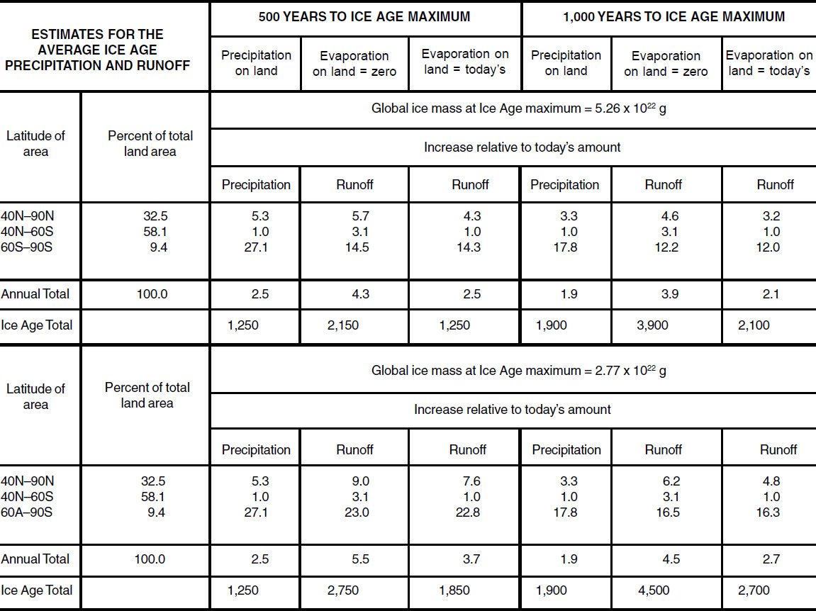
Table 1. Increases in precipitation and runoff calculated for two different Ice Age durations, global masses of ice, and evaporation levels on land. Each factor is the multiple of the present value in each category. Runoff estimates do not include deglaciation. See text for details.
The actual precipitation and runoff is time and location dependent and will vary substantially from the average annual values indicated in Table 1. Immediately after the Flood the ocean produced the greatest amount of precipitation and runoff, perhaps by a factor of 2 over that shown in Table 1. As the ocean cooled the precipitation and runoff decreased to about today’s level.
During the Ice Age precipitation increased in the 60S to 40N latitude zone, as evidenced by extinct river beds under the Sahara desert sands98,99 and elsewhere, and as alluded to in Genesis.
‘And Lot lifted up his eyes, and beheld all the plain of Jordan, that it was well watered every where, before the Lord destroyed Sodom and Gomorrah, even as the garden of the Lord, like the land of Egypt, as thou comest unto Zoar.’ Genesis 13:10 (KJV)
Today the plain of Jordan is not well watered, as it receives only 25 to 50 cm of rain per year. The inferred higher levels of precipitation (and runoff) in this zone are difficult to estimate, but would mainly be a redistribution of the increased precipitation proposed by Oard. The watersoaked sediments in this zone (at the end of the Flood) would contribute to evaporation above land and may increase early post-Flood precipitation in these areas. However, the global average Ice Age annual precipitation and runoff should be well within the extreme upper limits of the zero-evaporation model and calculations.
Precipitation and Runoff During Deglaciation
At the end of the Ice Age the ocean had cooled to near the present temperature, so the average precipitation approached that observed today. The precipitation distribution was likely different from today’s due to the presence of massive glaciers and vegetated areas (which are now deserts), and the resulting differences in albedo. Runoff in the Northern Hemisphere actually increased above earlier post-Flood levels due to the rapid melting of glaciers and ice sheets. This is indicated by the dramatic underfit nature of rivers in large channels that previously drained glaciated areas.
The underfit nature of rivers’ channels is determined by the present discharge rate as compared with the measured riverbed bankful width, depth, slope, and meander wavelength. Rapid melting during deglaciation produced tremendous runoff levels with cataclysmic erosion.100 The runoff rates, in the United States, during deglaciation may have averaged 18 times the present average runoff. Immediately south of the Laurentide glaciers, in Wisconsin, the rates may have been as high as 66 times the present rate.101,102
The minimum deglaciation time of peripheral portions of the Laurentide glaciers can be estimated by dividing the mass melting of ice draining into a river by the average annual carrying capacity of the river channel. The Mississippi River presently drains an area of 3.27 x 10⁶ km2 with an annual flow of 5.8 x 10¹⁷ g/yr.103 Approximately one-third of the Mississippi drain area was covered by Laurentide glaciers. The average thickness of Laurentide glaciers can be taken as proposed by Oard or calculated from the total ice mass and area covered by Ice Age glaciers. Melting glaciers draining into the Mississippi River system are assumed to have been one-half the average glacier thickness, since they were on the southern periphery of the largest glaciated area.
From the estimated mass of melting ice and the large runoff rates indicated by river channels, a minimum (and perhaps a maximum) duration for deglaciation of peripheral glaciers can be calculated. The results for various estimates of sea level changes, glacier thickness, and mass of snow and ice are shown in Table 2.104 These deglaciation duration estimates are in good agreement with Oard’s prediction of 50 to 87 years105 for the periphery of the ice sheets, which were derived from an entirely different approach.
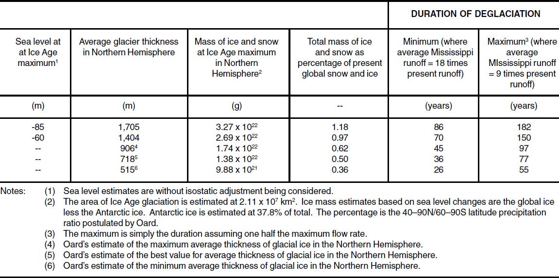
Table 2. Estimates of minimum and maximum duration of deglaciation. See text for details.
The average runoff during deglaciation is the total mass of melting snow and ice divided by the duration of deglaciation. It is generally assumed that the glaciers in Greenland and Antarctica would grow rather than melt during this time, so they can be excluded from these calculations. The runoff within the 40N to 60S latitude will be set to the present level, since Ice Age snow and ice in these areas are relatively small, as compared to the massive glaciers. Calculations show the global average runoff rates for the deglaciation of the 40N to 90N region range from 19 to 39 times the present level for the minimum and maximum durations of deglaciation (and corresponding mass of ice) in Table 2. These values are greater than the Mississippi runoff level, because the Mississippi drained a small portion of the melting Laurentide glaciers.
Post Deglaciation Precipitation and Runoff
The average annual global precipitation is controlled by the ocean temperature and heat input from the sun. From historic records, ice cores, and from the geologic evidence (that is, the Holocene interval) there is little reason to believe there has been a serious change in precipitation or runoff since the Ice Age deglaciation. Therefore post-deglaciation average precipitation is expected to be similar to today’s level.
Post-Flood Sediment Estimates
One could examine the total sediment moved and redeposited on the continents and in the sea to determine limits on the Flood/post-Flood boundary. The present rates of reworking sediment by erosion and redeposition on the continents has not been quantitatively estimated. So no real correlation between precipitation, runoff, and sediment redeposition (on the continents) is known. However, sediment arriving at the ocean is not likely to return to the continent, and if it is reworked by ocean waves and currents it will still be identified as marine sediment. Therefore, the following discussion will focus on the quantity of sediment arriving at the sea, sea sediment being all sediment deposited below the present sea level.
Post-Flood marine sediment can be divided into three groups based on the time of deposition:–
- (1) sediment deposited during the Ice Age,
- (2) sediment deposited during deglaciation, and
- (3) sediment deposited after the period of deglaciation.
Ice Age marine sediment must be estimated from post-Flood continental precipitation and runoff rates. Deglaciation and post-deglaciation marine sediments can be determined stratigraphically and estimated based on marine sediment studies. Post-deglaciation sediments are Holocene marine sediments.
Ice Age Marine Sediments
The mass of Ice Age marine sediments, that is, those that are post-Flood and pre-deglaciation, can be estimated from Ice Age runoff rates and the resulting continental erosion. Runoff rates were at their maximum immediately after the Flood and decreased, probably exponentially, as a function of time after the Flood. For simplicity, and because a model for the exponential decay of precipitation has not been developed, the runoff will be modelled as a linear decrease to the present level.
Present rivers, as supplied by present precipitation levels, carry about 1.6 to 2.0 x 10¹⁶ g/yr of solid and dissolved material to the ocean.106,107 This average is presumably about twice the rate of erosion before extensive farming began.
At the end of the Flood the vegetation cover, where present, was short with limited root penetration of the soil. There were only a few months of growth available late in the year of the Flood. The ground was not dry until the 314th day and everyone left the Ark 57 days later.108 It is not clear whether God regionally or globally delayed major rains during this time, to allow plants to grow to become food for animals, or the rains began even as the waters were receding off the continents. Vardiman’s post-Flood climatic model predicts a relatively low precipitation region at the east end of the Mediterranean across the continent of Asia.109 However, his model produces very cold temperatures in this region as well.
Barren land, ≤20 per cent vegetation cover, has an erosion rate about five times greater than land with a vegetation cover of 60 per cent or more.110 However, frozen ground, as predicted by Vardiman’s climatic model, does not erode very fast. In either case much of what is eroded is deposited downstream prior to reaching the sea.
Relating sediment load to runoff during a flood is not straightforward and has been the subject of many studies, resulting in numerous equations describing various relationships.111 Even with these studies, it is not clear how the models of short term high flow rates, well above normal flow rates, would correlate to the Ice Age situation where the runoff rates were high and the river channels were large and matched to the flow. A better approach would be to examine the variation of river sediment load as a function of the size and type of river. From this a method of scaling up to Ice Age runoff rates could be established.
Milliman and Syvitski recently analysed data for 280 rivers to characterise the loads and yields. There were 152 rivers with adequate data to find a good fitting equation relating sediment yield to runoff.112 The equation is
Y=aZb
where Y is the annual load per drain area (tons/km2-yr), Z is the average annual runoff per unit area (mm/yr) over the drain area, and a and b are constants. The constants have different values depending on the class of the river.
A summary of the river characteristics, number of rivers, annual loads, runoff rates, etc. from Milliman and Syvitski is given in Table 3. The table shows that the equations were used for rivers with runoff magnitudes that varied tremendously, by factors as large as 200 to 2,000 times. Since the equation characterises the nature of existing rivers with widely varying runoff rates, they should be reasonably accurate in predicting changes in sediment load resulting from an increased average runoff.
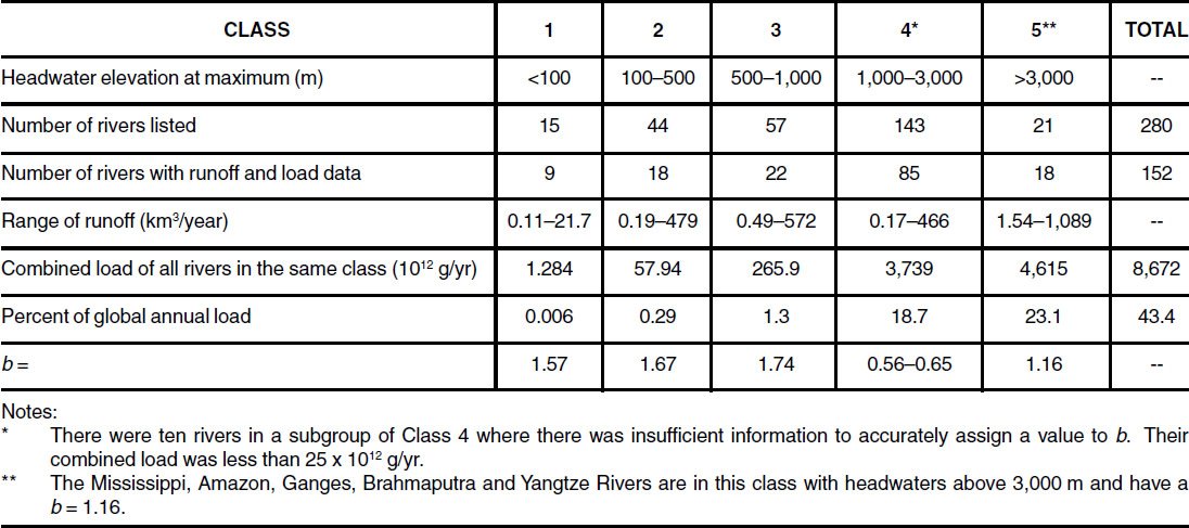
Table 3. River characteristics and constant b.
It is interesting that the majority of sediment is carried by rivers listed in Table 3 that have b ≤ 1.16. Where b >1 the load increases faster than the runoff, and where b <1 the load decreases as the runoff increases.
From the equation relating yield to runoff per unit area one can derive an equation relating a change in annual river load (g/yr) to the change in its runoff, making the reasonable assumption that there has been little or no change in the drain area. The equation is
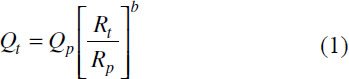
where Qt is the new load associated with Rt the new runoff, and Qp is the present load associated with Rp the present runoff, and b is a constant which can have one of six different values as shown in Table 3.
The linear decrease in runoff as a function of time after the Flood can be described by the following equation:
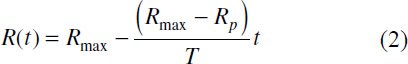
for 0 < t < T, and where

where Rmax is the maximum Ice Age runoff, Rave is the average Ice Age runoff, Rp is the present runoff, T is the duration of the Ice Age, and t is time in years after the Flood.
Combining the two equations gives the load as a function of time after the Flood. Integrating the equation gives the total mass M delivered over the duration of the Ice Age.
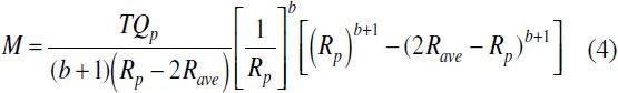
This equation describes the total sediment from a river where the present annual runoff and load is known. The equation also equally describes the total sediment from a number of rivers if Qp is the combined load from all the rivers, each river having the same increase in runoff, and each river having the same value of b.
During the Ice Age many rivers flowed that now do not; for example, those that are now under the desert sands, and Arctic or Antarctic ice. And midway through the Ice Age some rivers that flowed were stopped by glacial ice. These many changes are difficult to model, but an upper limit can be estimated.
To estimate the upper limit of Ice Age sediment carried to the ocean, the following assumptions can be made:
- (1) The Earth will be treated as a whole, with all the rivers lumped together.
- (2) The present annual global load of sediment delivered to the ocean, 2 x 10¹⁶ g, will be used for Qp.
- (3) The maximum value of the constant b will be used, that is, b = 1.74.
- (4) The maximum average Ice Age runoff Rave, in Table 1 for the 40–90N latitude and 1,000 year Ice Age, will be taken as the maximum. That is, 6.2 times the present runoff will be applied to the whole Earth. [This is a significant exaggeration as most of the land (58 per cent) falls within the 60S to 40N latitude which is expected to have a much lower runoff, between 1.0 and 3.1. Although the runoff in the 60–90S latitude is the greatest, it includes only Antarctica (nine per cent of the land surface). Applying an average runoff factor of 6.2 to the whole Earth and a b of 1.74 to all rivers should more than compensate any load losses in Antarctica, as it would require an increase in precipitation above the earlier estimates for the Ice Age.]
For T = 1,000 years, the total load M delivered to the ocean is calculated at 5.03 x 10²⁰ g. This is about 25,000 times the present annual load. Unfortunately this enormous number cannot be checked against some other method of independent estimation. The estimation is not unreasonably large as the ratio of sediment to water, by mass, is about 1.5 per cent or 30 times the present global average.
Similar calculations were made for other runoff levels and Ice Age durations. The results are summarised in Table 4. All the calculated values are within a factor of about two and one half of each other, indicating a dramatic change would be required to produce significantly more sediment during the Ice Age.
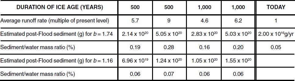
Table 4. Estimations of Ice Age marine sediment mass based for various runoff rates and Ice Age durations. See text for detailed explanation. Evaporation on land has been set to zero to maximize runoff.
Applying the highest average runoff from the 40N–90N latitudes to all the Earth’s rivers, the highest value of the constant b, and assuming no land evaporation, greatly exaggerates the total Ice Age runoff and loads. The estimated value of 5.05 x 10²⁰ g should be taken as a high estimate, and certainly a maximum limit on the Ice Age sediment carried to the world’s oceans.
A more probable value of Ice Age marine sediment could be estimated with a lower value of b. Floods of major rivers usually redistribute continental sediment rather than carrying a proportionally larger amount of sediment to the ocean. This is because the sediment-carrying capacity of a river is primarily a function of the water speed; the lower the speed the lower the sediment-carrying capacity. As a river increases in size (as it gradually approaches the ocean) the average speed typically decreases and sediment drops out.
The 1993 Mississippi River flood of North America was a good example of major flooding not dramatically increasing sediment discharge. This flood was notable for its high magnitude, long duration, and low sediment discharge. Times of peak suspended sediment corresponded to discharge levels at about two to three times the normal level. When the Mississippi exceeded this larger discharge level, reaching as high as about eight times its normal value, the suspended sediment dropped to a value more typical of, or below, the non-flooding level.113
With these considerations in mind a more probable estimate of Ice Age erosion can be calculated. The data in Table 3 shows that the majority of sediment is carried by rivers with a b < 1.16. Substituting the value of b = 1.16 into equation (4) one obtains a maximum estimate of Ice Age marine sediment at 1.55 x 10²⁰ g or about 15,000 times the present annual load. This would place the Flood/post- Flood boundary very late in the Pleistocene.
Deglaciation Sediments
The end of the Ice Age was a period of rapid deglaciation and massive catastrophic erosion. During the deglaciation, estimated by some to last a 3,000 radioisotope year interval, the Mississippi is believed to have supplied 1.5 x 10¹⁹ g of sediment to the Gulf of Mexico.114 This is about 1,000 times the current annual sediment carried to the ocean by all the world’s rivers. Areas other than the Mississippi delta also show massive erosion that resulted from deglaciation.
The global amount of ocean sediment produced by deglaciation can be estimated by assuming all glaciated areas responded like the Mississippi and that sediment carried to the ocean is proportional to the volume of meltwater runoff. The Mississippi is estimated to have carried the meltwater from 2.58 per cent of the northern hemisphere glaciers based on the prior estimates of glacial thickness and area covered by the Laurentide glaciers. Southern hemisphere glaciers are essentially those of Antarctica, which did not decrease in size during the deglaciation. The total amount of ocean sediment due to deglaciation is then estimated at 5.8 x 10²⁰ g.
Holocene Sediments
Post-deglaciation or Holocene ocean sediments can be estimated from Quaternary sedimentation data provided by Hay. Hay estimates the total marine sediment for the Holocene at 4.6 x 10¹⁹ g.
Flood/post-Flood Boundary Location as Determined by post-Flood Sediments
Combining the maximum Ice Age and deglaciation sediments with erosion since the end of the Ice Age (4,500 years times 2.0 x 10¹⁶ g/yr) gives a total post-Flood sediment of about 1.2 x 10²¹ g. This is about one twentieth of the total non-carbonate Quaternary marine sediments, which has been estimated at 24.71 x 10²¹ g by Hay. This sediment estimate places the Flood/post-Flood boundary very late in the Pleistocene, assuming a linear rate of marine sediment deposition in the Pleistocene.
Earlier placement of the boundary requires greater precipitation, erosion, and/or time. Placing the boundary at the end of the Mesozoic requires carrying to the ocean 4.38 x 10²³ g of sediment, less the biogenic and volcanic aircarried portions. This is nearly 400 times greater than the upper post-Flood limit estimated above. In addition, 1.69 x 10²³ g of sediment would have to be eroded and re-deposited on the continents. These quantities represent about 25 per cent of the total Phanerozoic sediment.
Placement of the boundary at the end of the Mesozoic would require incredibly severe post-Flood erosion. It would take over 10,000 years at 220 times (or 100,000 years at 22 times) the present annual global runoff to move 4.38 x 10²³ g of sediment. The required precipitation level to produce this much runoff is so high that all the land surfaces would be in a constant and tremendous downpour of rain. Terrestrial plants would find survival difficult, if not impossible, in such a wet environment. The cloud cover required to supply this much precipitation would make seeing the stars, Moon, Sun, and even a rainbow, a rare event.
Placement of the Flood/post-Flood boundary at the end of the Palaeozoic requires post-Flood upheavals and erosion of staggering proportions that approach those of the Flood. There are 8.77 x 10²³ g of existing Palaeozoic sediment, whereas 14.39 x 10²³ g of sediment are Mesozoic and Cainozoic. A Palaeozoic/Mesozoic boundary for the Flood would require post-Flood catastrophism to move 62 per cent of the entire Flood sediments (assuming all Phanerozoic sediments were originally Palaeozoic [Flood] sediments and there has been no loss of ocean sediments by subduction). This level of catastrophism, erosion, and sedimentation does not seem plausible during the Ice Age or in any biblically constrained time-frame, except during the year of the Genesis Flood.
Isostatic and tectonic adjustments that could affect the estimate of post-Flood marine sediment have been ignored for the following reasons:
- (1) Scripture indicates the land was dry at the end of the Flood and that the bound God placed on the sea would not be transgressed. (This is discussed in detail in a subsequent section.) A sea level that does not transgress this bound by rising relative to the continents severely limits any isostatic and tectonic adjustments.
- (2) A rising of the continents, or lowering of the sea level, would be consistent with Scripture, but would result in a net transfer of sediment from the continental shelf (ocean) category to the continental (dry land) category. Since most river-carried sediment is deposited at the mouths of the rivers and on the continental shelves, allowing a rise in continents would only reduce the estimated post-Flood-generated sediment found in the oceans.
Volcanism and Climatic Impact
Volcanism can dramatically affect post-Flood life through its climatic impact. Too much volcanism can block sunlight and destroy the majority, if not all, life on Earth. A significant, but smaller, amount of volcanism can produce cool summers, prevent crops from ripening, and make survival very difficult. Consequently, there is a limit to the amount of volcanism that can occur after the Flood. By comparing plausible amounts of post-Flood volcanism with the geologic distribution of volcanics, limits can be placed on the Flood/post-Flood boundary.
The historical record with the most severe account of extended attenuation of solar light occurred in AD 536– 537.115 A writer in Mesopotamia described the event as follows:
‘the sun was dark and its darkness lasted for eighteen months; each day it shone for about four hours, and still this light was only a feeble shadow . . . the fruits did not ripen and the wine tasted like sour grapes.’
Winters in Mesopotamia were very severe. In Italy, the summer of AD 536, Senator Cassiodorus wrote the following description:
‘The sun . . . seems to have lost its wonted light, and appears of a bluish color. We marvel to see no shadows of our bodies at noon, to feel the mighty vigor of the sun’s heat wasted into feebleness, and the phenomena which accompany a transitory eclipse prolonged through almost a whole year . . . a spring without mildness and a summer without heat . . . the months which should have been maturing the crops have been chilled by north winds . . . rain is denied . . . the reaper fears new frosts.’
The crops were killed off in Italy and Mesopotamia by cold and drought which led to severe famine in the following years. Similar effects were observed in China. Though the volcanic eruption causing the sun’s dimness has not been positively identified (it may have been Rabaul, on an island off New Guinea), this historic account demonstrates the serious climatic consequences of low light levels.
A similar dimming of the Sun was reported in 44 BC and is attributed to the explosive eruption of Mt Etna.116 Plutarch describes it as follows:
‘For during all that year its orb rose pale and without radiance, while the heat that came down from it was slight and ineffectual, so that the air in its circulation was dark and heavy owing to the feebleness of the warmth that penetrated, and the fruits, imperfect and half ripe, withered away and shriveled up on account of the coldness of the atmosphere.’
Atmospheric effects were also noted in China, where frost killed crops and there was widespread famine.
In view of the severe climatic consequences of volcanic eruptions only a limited amount of the Phanerozoic volcanic activity could have occurred during the 4,500 years since the Flood. A limit on post-Flood volcanism can be inferred from:
- (1) the total amount of volcanics in the Phanerozoic,
- (2) the volcanic eruption record in ice cores from Greenland and Antarctica,
- (3) limits on survivability due to volcanic-induced low sunlight levels, and
- (4) Scripture’s account of post-Flood life compared to volcanic-induced climatic conditions.
Volcanics in the Phanerozoic
The geologic record shows massive amounts of violent volcanic activity (see Figure 5). Volcanics represent at least 17 per cent of the continental Phanerozoic sediments. An annual eruption yielding a tiny fraction of these volcanics would result in a global climatic catastrophe.
Well known large flood basalts individually represent a small percentage of the Phanerozoic volcanics. A few of these are listed in Table 5.117,118,119,120,121,122,123 In comparison, Mauna Loa, Hawaii, a volcanic mountain which stands 6.6 km above the ocean floor, has a volume of 2.6 x 10⁵ km3 and represents 0.27 per cent of the volcanics.124 This gives one an appreciation for how common and massive volcanics are within the Phanerozoic.
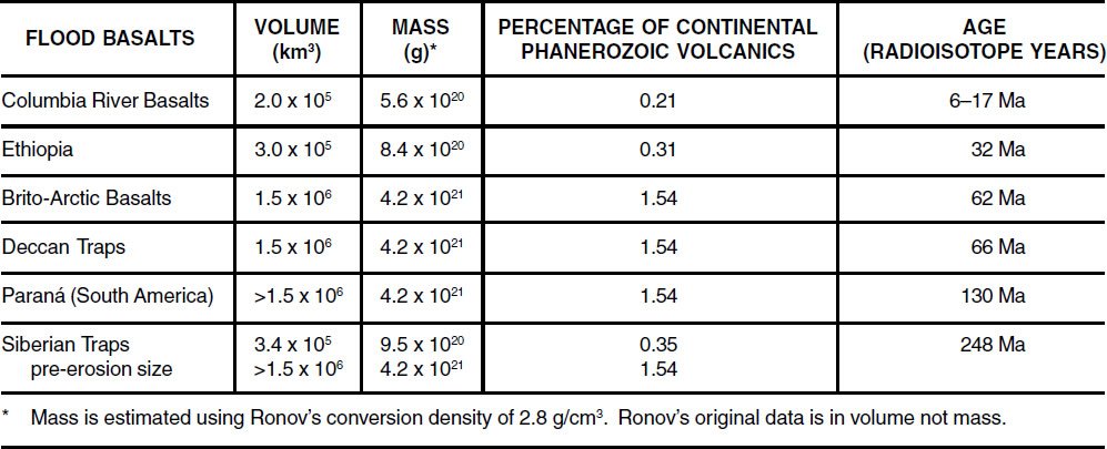
Table 5. Size of large continental flood basalts in order of radioisotope age.
The data for the Phanerozoic volcanics, less the Quaternary, is based on several decades of work by A. B. Ronov and others,125,126,127,128,129 previously discussed. The Quaternary estimate is based on research by others.
No attempt has been made to adjust the amounts in Figure 5 to account for volcanics lost to erosion. Some estimates of erosion indicate a repeated reworking of sediments on a massive scale.130,131 These erosion estimates indicate that the volcanics shown in Figure 5 are dramatically underestimated, with the actual volcanics being more than twice that shown. Massive erosion and redeposition is indicated by the many large-scale unconformities throughout the geologic column.
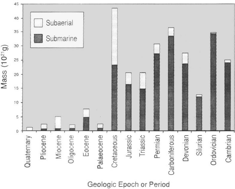
Figure 5. Distribution of Phanerozoic continental volcanics.
There was legitimate criticism of Ronov’s earlier compilation;132 however, the data have been revised. A summary of the revised data,133 when compared to earlier summaries, shows significant changes in the distribution of continental volcanics within the Triassic, and among the Cambrian through Devonian periods. The net change has been a reduction of Phanerozoic, non-Quaternary, continental volcanics by seven per cent to a total of 272 x 1021 g. Inclusion of volcanics from continental shelves and slopes, and ocean floors, adds 84 x 1021 g (31 per cent) and 8 x 10²¹ g (three per cent), respectively, giving a total of 364 x 1021 g. These marine volcanics are not shown in Figure 5.
The summary did not subdivide continental volcanics into terrestrial and marine categories. To provide a terrestrial and marine distribution of volcanics in light of the revision, the continental volcanics data were pro-rated according to the terrestrial and marine subdivisions of Ronov’s earlier work.134 This is the Phanerozoic, non-Quaternary, data presented in Figure 5. In view of trying to determine where the Flood/post-Flood boundary is located, terrestrial volcanics will be described as subaerial and marine volcanics as submarine.
Determinations of subaerial or submarine volcanics are generally based on the presence of pillow lavas and/or the facies of interbedding sediments. Pillow lava is indicative of the presence of water independent of whether the water is the Flood of Genesis, post-Flood inland lakes, or the ocean. The absence of pillow lava is not so clear an indicator of subaerial environments, as pillow lava formation is dependent on extrusion rates and melt viscosity.135 Pillow lava has been observed only on the edges of rapidly extruded submarine sheet flows,136 which sometimes resemble subaerial pahoehoe toes.137 This is important for Flood and post-Flood models considerations, since the absence of pillow lavas could incorrectly lead one to conclude that flows were subaerial. I have not attempted to reclassify Ronov’s submarine and terrestrial volcanics, as it is beyond the scope of this investigation.
The total Quaternary volcanics is my estimate based on the work of several researchers. Decker138 provides an estimate of the number of eruptions for all sizes of volcanic eruptions for the last 1 million radioisotope years. This data is based on an extrapolation of 10 years (1975–1985) of detailed eruption records,139 historical records of large eruptions during the last 200 years, and a listing of the known 209 large calderas of the world that were formed during the last 2 million radioisotope years.140 All Quaternary volcanics are assumed to be subaerial because the sea level throughout the Quaternary was between +35 m and -85 m of the present sea level according to the Vail curve.141
Using Decker’s eruption size and frequency estimates, the mass of Quaternary volcanics is calculated at 1.3 x 10²¹ g. Figure 5 shows this quantity of volcanics. This is about 10 per cent of the total Quaternary continental sediments estimated by Hay.142 In comparison, Ronov estimated 1.73 x 10²¹ g of volcanics for the Pleistocene.
Eruption of subaerial volcanoes, which generate fine ash and aerosols, are the only ones that directly affect sunlight transmission and Earth’s climate. Consequently, subaerial volcanics, which represent 21 per cent of the Phanerozoic volcanics, will be the primary focus for further consideration. The effects of submarine volcanic eruptions are mitigated by water that absorbs ejecta, ash, aerosols, and heat.
Ice Core Records
Ice core records contain a history of the Earth’s environment frozen in the polar ice sheets. Dust and gases thrown into the stratosphere from volcanoes migrate to the polar regions, where eventually they are incorporated into the precipitation of the region. Ice cores record variations in acidity, volcanic and wind blown dust, changes in the ratio of 16O/18O (δ18O), etc., during the time of precipitation. Diffusion, migration, melting, percolation, and re-freezing can distort the record, but important clues to Earth’s meteorological past remain. If the core records go back far enough, limits on post-Flood volcanism, both in time and magnitude, can be determined.
Oard has indicated that areas of high elevation on Greenland and Antarctica (that is, mountains and East Antarctica) would accumulate snow rapidly in the Ice Age, whereas lower elevation areas would accumulate ice more slowly.143 Antarctica was expected to have an average of 1200 m of ice by Ice Age maximum, with the majority of the ice on East Antarctica. Greenland would have had about 700 m of ice at the same time. This suggests that ice cores from Greenland and Antarctica could extend well into the Ice Age if taken from elevated areas, assuming the early snow record has not been lost in distortion, thinning, melting, erosion, etc., which commonly occurs.
Ice cores from Camp Century, north-west Greenland, and Byrd Station, West Antarctica, were not drilled over high elevation areas, but were drilled over areas where the base of the ice sheet was generally low in elevation. The elevation of the base of these cores are at 500 m above and 500 m below sea level, respectively.144 Other cores have been drilled over higher base elevations, but the drilling did not reach the base of the ice sheet.
The lower sections of these cores show two dramatic changes in δ18O (about -10 per cent), which indicate the beginning and end of the Ice Age in the old earth paradigm. Within the young earth paradigm, Vardiman has proposed that such changes are due to:
- (1) a change in distance between source and deposition of precipitation,
- (2) a change in concentration of δ18O at the source, or
- (3) a change in type of precipitation.145
He suggests these changes in δ18O are associated with a change in climate caused by a cooling of the post-Flood oceans. The first change may have been induced by the growth of polar ice shelves, and the second by the melting of the same ice shelves.
One can roughly estimate the duration of the ice core records by using the rapid climatic change recorded at the Ice Age end as a gauge. Oard indicates at the end of the Ice Age the periphery of the sheets would melt in 50 to 87 years, and the interior would melt within 200 years.146 Vardiman has suggested ice shelves melted in 40 years.147 Evolutionists have recently estimated a 7°C warming in South Greenland in 50 years and a rapid calming of the North Atlantic in only 20 years.148
Using the estimate of 40 years for the change in δ18O as a gauge, per Vardiman’s interpretation of melting ice shelves, one can roughly estimate the age of the earliest ice core records.149 In the Camp Century core, I interpret the dramatic change in δ18O from -38 per mil at 1,158 m to -30 per mil at 1,128 m as the rapid melting of the ice shelves in 40 years. This gives an estimated core-thickness-to-time ratio of 0.75 m per year. Extrapolating this to the lowest level gives a maximum age at the bottom of the Camp Century core (at 1,370 m); the age of ice at the bottom is estimated at about 280 years before the end of the Ice Age or about 700 years after the Flood, assuming a 1,000 year long Ice Age. This sets a limit of 700 years on the duration of volcanic activity where records are not available. The bottom of the Byrd Station core suffers from distortion and was therefore not used in these calculations.
If the Ice Age lasted only 500 years, there were only 220 years during which global volcanism was not recorded in the Camp Century ice core. Throughout the following discussion a 1,000 year Ice Age will be assumed, unless identified otherwise, to provide a significant length of time for volcanism that was not recorded in the ice cores.
Examination of the concentration of different dust particles in ice cores can give clues to the level of volcanic activity from 700 years after the Flood to the present.
‘The morphology and elemental composition of the particles indicate that two types of particles are dominant — volcanic debris and mineral dust. The particles in the Antarctic core (Byrd Station) are predominantly volcanic whereas those in the Greenland core (Camp Century) are predominantly soil-type minerals; at the latter site only about 5% of the particles are volcanic during the Wisconsin (Ice Age).’150
Examination of the dust or acidity throughout the cores from Camp Century,151,152 Dome C,153 Vostok154 and Byrd Station155,156 shows no evidence for significant global volcanism. Significant means:
- (1) eruptions having serious and lasting global effects, or
- (2) eruptions that would contribute to as little as 0.01 per cent of the subaerial Cainozoic volcanics.
If such eruptions had occurred they would have been detected, because the historically-large but geologicallyminor eruption of Tambora (1815) is evident in the cores, as are numerous older eruptions. Where the lower core sections record increases in dust, the significant increases are due to loess or from local volcanism.
The typical concentration of dust at Camp Century and Byrd Station is about 1 x 10⁴ particles per core section for particles larger than 0.62 micrometres.157 At Camp Century dust concentrations throughout the core are low, except around 1,200 m where the dust concentration jumped by a factor of 100; the dust at these areas of higher concentration is of non-volcanic origin. At Byrd Station the dust concentration increased by a small factor of four between 1,400 and 1,600 m, with low dust concentrations at higher and deeper levels; the dust is of volcanic origin at the peak concentration and is attributed to volcanoes on East Antarctica.158 In contrast to the Byrd Station core, other cores from Antarctica, Dome C159 and Vostok,160 have little dust of volcanic origin.
The low levels of volcanic dust or acidity from Camp Century, Byrd Station, Dome C, and Vostok indicate low levels of volcanic activity throughout the cores. These data limit the available time for serious post-Flood volcanism to sometime before the ice sheets began to grow. This duration is roughly estimated at 700 years, assuming a 1,000 year Ice Age, although it may have been only 200 years, assuming a 500 year long Ice Age.
Survivability During Reduced Sunlight Conditions
The limit of photosynthesis is at about 1 per cent of the Sun’s light, whereas continual cloudiness limits the transmission to about 10 per cent.161,162 A full moon gives about one millionth of the Sun’s light. It would seem that as a minimum the post-Flood environment needed light transmission levels at the 10 per cent level for vegetation to grow, and occasionally at much higher levels to make a rainbow visible.
The largest eruption in recent history was that of Tambora in 1815.163 Tambora ejected about 175 km3 of ash and pumice, and apparently cooled the Earth in the years following. Though there is some debate about the cooling effect of Tambora, 1816 was called the ‘year without a summer’. Many crops failed to ripen and the poor harvest led to famine, disease, and social distress.
Presumably the largest explosive eruption in the Quaternary was Toba (Sumatra) at about 75,000 radioisotope years ago.164 The estimated eruption volume exceeds 2,000 km3 of magma. Toba produced over 10 times the ejecta and 50 times the stratospheric aerosols of Tambora. Estimates of Toba’s effect indicate the light level would have been like that of a very cloudy day to below the limit for photosynthesis, depending on proximity to the eruption. The presence of clouds would have reduced light at the Earth’s surface to an even lower level.
Mt Curl (New Zealand) provided another very large Quaternary eruption and is dated at about 250,000 radioisotope years ago. The ash covered at least 107 km2, and the estimated volume of the eruption is from 1,200 to 2,200 km3.165 Its impact must have been comparable to Toba.
Flood basalts are thought to release an order of magnitude more sulphur volatiles (aerosols) than explosive eruptions of the same volume. Stratospheric aerosols greatly reduce the level of incoming sunlight and can have a severe impact on plant and animal life. The most recent and massive flood basalt was Roza (dated 14 million radioisotope years ago), which is part of the Columbia River Basalt Group. Roza produced about 700 km3 of basalt in seven days, and is estimated to have reduced the worldwide light level several orders of magnitude, well below the minimum level for photosynthesis.166
The Pliocene eruption in Yellowstone that produced Huckleberry Ridge Ash has a radioisotope age of 2 Ma and produced 2,450 km3 of tuff and ash.167 A more recent Pleistocene eruption in Yellowstone with a radioisotope date of about 620,000 years, produced the Lava Creek Ash with 1,000 km3 of tuff.168 The ash from these two eruptions covered 3 x 10⁶km2 and 4 x 10⁶km2, respectively.169 These eruptions would have had a serious climatic effect comparable to that of Toba.
The rate of post-Flood volcanism must be below the lethal level for Noah and his descendants to survive. The aerosols from a basalt flow like Roza could kill or prevent harvesting of plants for one year or more, and the effects of an explosive eruption like Toba would probably do the same. The average material erupting from these two volcanoes is about 1400 km3 or 4 x 10¹⁸ g. An annual eruption of this magnitude for decades or centuries should be considered a near-lethal level, if not absolutely lethal, since plants would not be able to produce under these conditions. Famine, disease, and death would prevail on land and sea under these conditions.
To estimate the maximum post-Flood volcanic material generation, post-Flood volcanism at the near-lethal level will be assumed. The rate will be set at one eruption per year, maximum. If this eruption rate and intensity continued for 700 years after the Flood, that is, roughly the duration of the Ice Age before ice core records begin, the total post- Flood volcanics would be a maximum of 2.8 x 10²¹ g. This amount is about 21 per cent of the subaerial Cainozoic volcanics shown in Figure 5. This estimated amount of volcanics would place the Flood/post-Flood boundary in the Early Pliocene. If much of the Pliocene and Pleistocene volcanics have been eroded away, the boundary location would be somewhat higher in the column.
The estimated maximum of 2.8 x 10²¹ g of global post- Flood volcanics is no doubt a great exaggeration, as a nearlethal level is severe and would eliminate the ripening and harvesting of most, if not all, crops and fruits on Earth. A more realistic estimate of the maximum post-Flood volcanism would be one-tenth (or less) of the near-lethal eruption level. This would approximate post-Flood volcanism at one Tambora-equivalent eruption every five years until the beginning of the Ice Age. This more reasonable level of volcanism for 700 years would reduce post-Flood volcanics to 2.8 x 10²⁰ g and place the Flood/ post-Flood boundary after the mid-Pleistocene. Assuming a 500 year long Ice Age and reasonable levels of volcanism would reduce the post-Flood volcanics to about 8 x 10¹⁹ g and place the boundary very late in the Pleistocene.
Scripture’s Account of Post-Flood Life
A dark Earth does not appear to be the kind of world Noah and his descendants lived in. The post-Flood world was meant to be inhabited and to bring forth vegetation. The animals were to go forth, breed abundantly, and refill the Earth (Genesis 8:15-17; 9:1). For animals to leave the Ark and survive would require sufficient vegetation for all to eat. [Future carnivores must have been eating plants or numerous herbivore kinds would have been lost during the first few decades after the Flood.] To grow an adequate supply of vegetation, there must have been sufficient sunlight for the preceding months, prior to the end of the Flood. It would seem strange for God to go to the trouble of saving animals on the Ark, only to have them all perish for lack of food after the Flood.
The fresh olive leaf (Genesis 8:11) indicates there was ample sunlight for plant growth during the last few months of the year of the Flood. The Scripture also speaks of sufficiently bright sunlight to produce a rainbow (Genesis 9:12–17). The atmospheric effects of late-Flood volcanism appear to be minimal according to Scripture’s account.
The years immediately following the Flood appear to have had plenty of sunlight. Grapes require lots of sunlight, and Noah apparently had a bountiful crop of grapes. Later Nimrod was described as a mighty hunter (animals must have been alive and well), and people were doing well enough to spend extra time building the Tower of Babel. This requires ample food, good harvests, and significant sunlight. The climatic effects of late-Flood and post-Flood volcanism appear to have been minimal according to Scripture’s account.
Earlier Placement of the Flood/post-Flood Boundary
Placing the Flood/post-Flood boundary lower than the Pleistocene would require some mechanism to continually cleanse the atmosphere (high into the stratosphere) of aerosols and ash during a time of great volcanism. Mechanisms available to do this appear to be inadequate or near miraculous.
Rain and snow are ineffective in cleansing the atmosphere of explosive volcanic emissions because most clouds reside in the troposphere, below 13 km, whereas explosive volcanic ejecta send dust and aerosols well above this height into the stratosphere, 13–47 km. The Mt St Helens eruption of 1980, with 1 km3 of ejecta, was a very small eruption, yet the eruptive column reached over 25 km.170 The much larger eruptive columns of Krakatoa in 1883 and Tambora in 1815 are estimated to have reached a height of 40 km.171,172 Visible affects of Krakatoa lasted about a year and that of Tambora173 for over two years. The small eruptions of El Chichon (1982) and Pinatubo (1991) individually increased the stratospheric aerosols by over an order of magnitude; the aerosols lasted about a year and a half at this concentration.174 Rain and snow did not immediately clear the atmosphere of aerosols from these volcanic eruptions and would not immediately clear aerosols from explosive eruptions after the Flood.
Rain and snow are only slightly effective against the effects of aerosols from flood basalts, as is demonstrated by the summer 1783 eruption of Laki (Iceland).175 Laki was the most active during the first two months (June and July) of an eight-month-long eruption that produced a mere 12.3 km3 of lava. The haze in Europe was worse during June and July and was not affected by changing wind directions; this indicates the aerosols had reached the upper troposphere. The haze was essentially gone by December 1783, indicating the aerosols had, for the most part, been retained in the troposphere. Even though the haze was shortlived, the aerosols from Laki appear to have caused the coldest winter in the Northern Hemisphere in 225 years, being 4.8°C below the long term average. Mean temperatures for the spring, autumn, and winter of 1784 and 1785 were also below normal. Small flows of flood basalt like Laki have severe environmental effects in spite of rain or snow.
An impact of a large asteroid could inject substantial water into the stratosphere and potentially wash out aerosols.176 However, the accompanying catastrophism would be worse than the volcanism that produced the aerosols.177,178 Consequently, this is not a solution to cleaning the stratosphere of aerosols.
One could suggest volcanic-like explosive eruptions could somehow shoot ocean waters, that have little ash or aerosols, high into the stratosphere to cleanse the atmosphere. But creating a credible scenario that can do this seems miraculous in itself. One could also suggest a continual influx of ice particles from comets that are mostly ice; however, the timing and availability of a continual source of comets sufficient to cleanse the atmosphere often enough (yearly or more often) for 700 years after the Flood seems equally miraculous.
All scenarios that cleanse the atmosphere after the Flood must do so continually, or at least on a frequently repeated basis. Serious volcanism for even a few years in a row would decimate post-Flood plant, animal, and human life. The serious climatic effects of continued volcanic eruptions seem to make the challenge of having significant post-Flood volcanism very difficult to overcome.
Volcanism and Climatic Impact Summary
The maximum post-Flood volcanism would have produced 2.8 x 10²¹ g of volcanics. This quantity, when compared to the estimated amount of volcanics in the strata, places the Flood/post-Flood boundary in the Early Pliocene at the earliest. A less dramatic and more reasonable amount of post-Flood volcanism during a 1,000 year Ice Age would be one tenth, or less, of the estimated value and would place the boundary after the mid-Pleistocene. A 500 year Ice Age and a reasonable amount of post-Flood volcanism reduces the volcanics to 8 x 10¹⁹ g and places the boundary very late in the Pleistocene.
It is not clear how one could place the Flood/post-Flood boundary earlier than the mid-Pleistocene; to do so would compress tremendous amounts of volcanism into only 700 years after the Flood. This would cause mass mortality when animals and man are to be scattered and filling the Earth (Genesis 8:15–17; 9:1). It is also not apparent how an environment could be constructed to cope with tremendous post-Flood volcanism without re-opening the windows of heaven to continually purge the atmosphere of volcanic dust and aerosols. Proposing significant volcanism in the post- Flood world would seem to make post-Flood survival as miraculous as the survival of Noah and the animals on the Ark.
Obviously something cleaned the Earth’s atmosphere of volcanic particles and aerosols generated during the tremendous volcanic events of the Flood. Perhaps one of the purposes for the waters from the ‘windows of heaven’ (Genesis 7:11–12) was to clean the atmosphere in preparation for post-Flood life.
If the terrestrial volcanics have been accurately identified, major terrestrial eruptions would have to have been completed prior to stopping the windows of heaven on the 150th day of the Flood (Genesis 7:24; 8:1–4). If this interpretation is correct, the 150th day of the Flood would be late during, or after, the mid-Pliocene; the Flood/post- Flood boundary could be no earlier.179 This also implies that the receding of Flood waters after the 150th day would have eroded much of the late Cainozoic strata, and exposed earlier deposited strata.
There may have been Flood sediments above the Miocene and Pliocene that were eroded during the last seven months of the Flood. Such sedimentary layers were alluded to by Nelson180 as those containing pre- Flood man. We have no continental record of these sediments or they have been mis-identified. The fossil content of these sediments would have been similar to Miocene and Pliocene fossils, except that human fossils might have been common. These sediments, if they existed, could be placed in a geologic era I call ‘Erodeozoic’, meaning eroded life. If the Erodeozoic was real, the 150th day of the Flood would correspond to the top of the Erodeozoic. Erosion after the 150th day would remove most or all of the Erodeozoic sediment to the sea, effectively moving the Flood/post-Flood boundary deeper in the geologic column to the Pliocene or Pleistocene epochs. If the Erodeozoic hypothesis has validity, one would expect these layers could be found in enclosed basins where they would not have been lost.
A straightforward interpretation of the biblical account, in view of the climatic impact of volcanism, places the Flood/post-Flood boundary extremely late in the Cainozoic. Without some effective and continual method to cleanse the post-Flood atmosphere of volcanic aerosols and dust, one is compelled to place the Flood/post-Flood boundary very late in the geologic column. The evidence from maximum plausible post-Flood volcanism places the Flood/post-Flood boundary during or after the Early Pliocene. Reasonable amounts of post-Flood volcanism place the boundary after the mid- Pleistocene.
Formation of the Mountains of Ararat
If one can geologically date or put stratigraphic limits on the formation of the Mountains of Ararat, then the 150th day of the Flood can be geologically dated. Because the end of the year of the Flood was 221 days after the Ark came to rest, the Flood/post-Flood boundary must be younger than the Mountains of Ararat.
Scripture states that the Ark came to rest in the ‘Mountains of Ararat’ on the 150th day of the Flood. The Ark stayed on these mountains for the remaining 221 days of the Flood year. In supporting the Ark, the mountains survived the last 221 days of Flood activity, including massive erosion as the waters receded off the face of the ground and contemporaneous volcanism. Late-Flood erosion must have been the most destructive global process after the 150th day of the Flood; nothing of comparable magnitude of destruction has happened since or will until the end of the age (Genesis 8:21; 9:11, 15; 2 Peter 3:7, 12; and Revelation 16:18; 21:1). Another worldwide flood would be required to produce a comparable amount of erosion.
If the Mountains of Ararat survived the massive erosion after the 150th day of the Flood, then one would expect the mountains to survive all post-Flood destruction—excepting possible post-Flood major volcanic eruptions and/or major earthquakes. Therefore the original Mountains of Ararat should exist today, or at least significant remnants.
There are good reasons for Scripture referring to the Mountains (plural) of Ararat. A group or chain of mountains would be required to form a safe ‘harbour’ for the landing of the Ark. Without a harbour or direct divine protection, the tumultuous receding Flood waters would break the Ark on landing as tremendous waves crashed upon the rising mountains. A group or chain of mountains would create breakers to mitigate the violence of waves and form a protected area for safe landing of the Ark. Any post-Flood catastrophism would have to be tremendous to destroy a group or chain of mountains specifically designed to bring the Ark to safe landing during the Earth’s most violent catastrophic flood. It seems more likely than not that the Mountains of Ararat would have survived well into post- Flood times, considering the biblical reference to mountains (plural) and the implications for a group or chain of mountains.
Ancient historians claim remains of the Ark were existing in the Mountains of Ararat into their day. These historians include Berosus the Chaldean, Hieronymus the Egyptian, Nicolas of Damascus, and Josephus.181 These historians wrote from what appears to be second-hand information, but did so in a matter-of-fact manner, as if remains of the Ark were common knowledge. If these accounts have any merit, they imply that the Mountains of Ararat were not destroyed by post-Flood catastrophism but survived well into post-Flood time and exist today. These historical accounts, and the need for stable and enduring mountains, indicate that one only needs to determine the geologic age of existing mountains to determine the geologic age of the 150th day of the Flood. This greatly reduces the range and scope of geologic issues to be considered.
The Land of Ararat —Urartu
The Hebrew word translated as Ararat in Genesis 8:4 appears to be the name of a country, and is so rendered in Isaiah 37:38. Historically, Ararat has been associated with the ancient land of Armenia.182 The predecessors of the Armenians are the people of the kingdom of Urartu. Urartu is an Assyrian name and the Urartuians called their country Biainili.183 The kingdom of Urartu covered the area shown in Figure 6, and had its geographical centre near Lake Van (elevation 1646 m). I have enlarged the generally accepted size of Urartu to include all nearby mountains so as to include all possible Mountains of Ararat. The aim is not to solve this great mystery, that is, identify the true Mountains of Ararat as others have attempted,184 but rather to put reasonable geographic limits on the possibilities on the mountains of Urartu, and set geologic limits on the Flood/ post-Flood boundary.
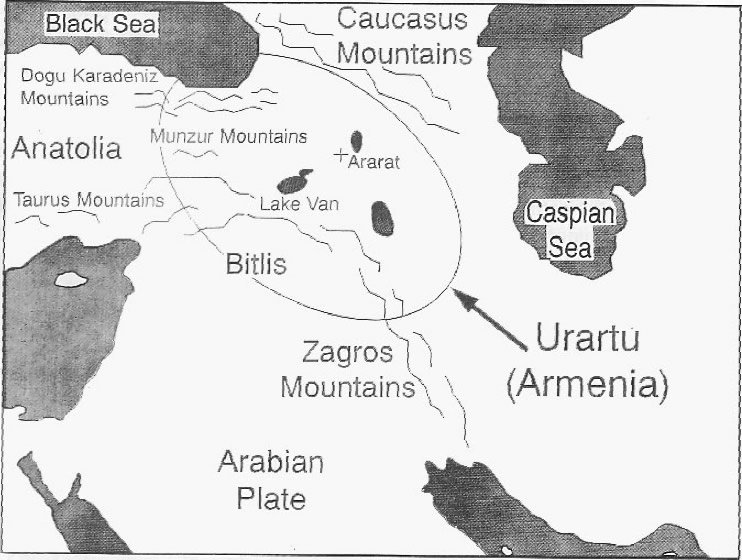
Figure 6. The land of Urartu or ancient Armenia.
In the broadest sense, the Mountains of Ararat could be any of the mountains of Urartu: the many volcanic mountains in the land of Urartu, the northern Zagros Mountains, the north-eastern Taurus Mountains, and the mountains in the Bitlis suture zone. Though not commonly thought to be part of Urartu, the enlarged geographical region includes the Dogu Karadeniz Mountains, the Munzur Mountains, and the southern edge of the Caucasus Mountains.
The geology of Urartu is complex and has been the subject of numerous studies. The geology is complex because it appears to be an area of repeated continental collisions, and includes many fragments thereof.185,186 Suffice to say:–
- (1) the geology is dominated by marine facies (limestones, pillow lavas, etc.) from Early Palaeozoic through the Mesozoic and into the Cainozoic, and ophiolite structures are present through the Cretaceous;
- (2) volcanics are present in the Mesozoic, but volcanic mountains were not formed until the Cainozoic;
- (3) during the Mesozoic the area was dominated by the Palaeotethys, Mesotethys, Tethys, and Neo-Tethys oceans; and
- (4) all significant mountain-building occurred during the very active Cainozoic.
Volcanic Mountains
Volcanic mountains, or cones, in central Urartu are dated from the Middle Miocene to the present.187 These volcanoes lie within an 800 x 300 km zone of Oligocene to Quaternary volcanic rocks and sediments which overlie older sediments. The region is covered with vast volcanic deposits interspersed with clastic sediments. If the Mountains of Ararat are volcanic in origin one would expect:
- (1) the mountains to have cooled somewhat and stabilised prior to the Ark coming to rest on them, and
- (2) limited volcanic activity in the area thereafter.
A wooden ark would not survive on a hot and fiery volcanic mountain apart from direct divine intervention. Man and animals cannot survive anywhere in an area where volcanism is intense and massive.
Volcanics are so extensive in the area that the Lake Van region had to be very dangerous when the volcanoes were erupting. Potassium-argon dates for volcanics in the area range from 0.7 to 13.1 Ma in radioisotope time.188 This places the flows between the mid-Miocene and the mid- Pleistocene.
The famous Mt Ararat in Turkey, where many go in search of Noah’s Ark, is the highest in a group of eight stratovolcanoes in the Iran-Armenia-Turkey border area.189 Mt Ararat is a large volcano. It covers 1,000 km2, is 5,156 m high, and has a volume of about 1,700 km3. The main structure of Ararat is made of two chemically distinct calcalkaline volcanics. The lower structure consists of calcalkaline andesite and is thought to have been generated under more hydrous conditions than the higher volcanics. The higher volcanics include andesite, dacite, and rhyodacite.
Flowing onto the main structure are fresh, later basalts which ‘can be clearly distinguished as black, soil-free flows on the flanks of the mountain.’ These fresh basalts ‘erupted from fissures in post-glacial time’.190
Ararat lies in an area of volcanics dated between the Lower Miocene and the present.191 Ararat appears to have been a very active volcano during the Quaternary.
Burdick has described the Mt Ararat region as follows:
‘Eastern Turkey consists of a relatively barren, undeveloped area, quite without tree cover. Tectonically, it is very active, and unstable structurally. The region has been folded, faulted, and intruded with basic types of volcanic rock such as andesite and basalt. Previously the cover rocks had been Paleozoic and Mesozoic limestone, but these have been eroded, folded and faulted by frequent orogenic activity, forming volcanic mountains, among which are the Tendurek Range, and also the Alogoz-Ararat system.’192
‘Apparently the Paleozoic-Mesozoic limestone complex which covered parts of the region was severely deformed, compressed, folded, and in places like the Ararat area domed up when the rising magma burst through. This doming effect is most evident when one views the same limestone formation on all sides of Mount Ararat. The beds dip away from the mountain on the Turkish, the Russian, and the Persian (Iranian) sides.’193
On Ararat itself one finds marine sediments as high as 14,000 feet (4,267 m).194 Devonian and Permian sediments are found on Ararat.195 Since the sediments are older than the formation of Ararat, they may have been carried to these heights as the volcanic dome of Ararat grew in size.
Burdick continues with the observation that different compositions, or least different textures and colours indicate
‘. . . the original Mount Ararat apparently was not more than from 10,000 to 12,000 feet in height. The present peak is about 17,000 feet, and at its greatest height perhaps measured nearer 20,000 feet. Erosion has worn it down.’196
He also notes that
‘When lava is extruded under water it is cooled quickly and solidifies so rapidly that crystals often have no time to form, like obsidian; or very small crystals are formed. Much of the basalt and andesite composing upper Ararat was of this type. The lava is often found in rounded blocks called pillow lava, because they are of pillow-like appearance having conchoidal fractures.’197
Burdick goes on to list invertebrate index and other fossils found in the limestones and sediments of the Dogubayazit-Igdir area (which includes Mt Ararat).198 These include fossils from limestones of the Devonian, Mississippian, Pennsylvanian, Permian, and Triassic. Fossils from unspecified sediment types are listed from the Jurassic (ammonites), Cretaceous, Eocene, Oligocene, and Pliocene. Many of these fossils indicate marine facies.
The Zagros and Taurus Mountains
The mountains in the southern portion of Urartu are a part of a band of mountains that include the Zagros and Taurus Mountain ranges. This band of mountains resulted from the collision of the Arabian plate with the Eurasian plate. The area of the collision is called the Bitlis/Zagros suture zone and extends from the Mediterranean Sea, just south of the Taurus Mountains, up through the middle of Urartu and down to the Persian Gulf (or Gulf of Arabia) by way of the Zagros Mountains.
This collision between the Arabian plate and Eurasia began in the Middle to Late Eocene, with major mountainbuilding starting in the Miocene. The collision was completed sometime between the Early Pliocene and the present.199 The Bitlis/Zagros suture began in the Middle to Late Eocene, with terminal suturing in the middle of the Miocene.200 Regional uplift of eastern Anatolia began in the Middle Miocene and was completed in the Early Pliocene. Uplift of the entire Anatolian-Persian Plateau also appears to have been completed by the Early Pliocene; this is indicated by a regional unconformity in the Early Pliocene in the Silvas Basin201 (in central Turkey) and in far eastern Turkey.202
Dogu Karadeniz Mountains
The Dogu Karadeniz Mountains are located south of the eastern end of the Black Sea, about 300 km north-west of Lake Van. They are part of the Pontides-Transcaucasus Mountains. During the Mesozoic these areas are described as magmatic or volcanic arcs, and are thought to have been very active. Cone formation seems to have been minor or absent. In the Late Palaeocene to Early Eocene the Anatolide-Tauride Platform collided with the Pontides, causing great deformation in the Anatolide-Tauride Platform and uplifting the Pontides.203 The Dogu Karadeniz Mountains appear to have reached their highest elevation in the Pliocene with the uplifting of Anatolia.
Marine environments dominated the Anatolide-Tauride Platform in the Middle to Late Miocene, with permanent subaerial facies of Anatolia beginning in the Pliocene.204 A massive Tertiary granite structure (over 150 km x 50 km) with volcanic intrusions makes up a significant portion of the Dogu Karadeniz Mountains, with peaks up to 3,560 m.205 The area would have been very dangerous in much of the Cainozoic.
Munzur Mountains
The Munzur Mountains (peaks to 3,188 m) lie on the western periphery of Urartu about 300 km from Lake Van, at the western end of Anatolia. They are thought to have risen above the surrounding ocean in the Early to Middle Eocene,206 and are made of deformed Mesozoic and Palaeozoic sediments. The Munzur Mountains, like the Dogu Karadeniz Mountains, appear to have reached their highest elevation in the Pliocene with the uplifting of Anatolia.207 Although near the land of Urartu, the Munzur Mountains are not commonly thought to be part of Urartu.
Caucasus Mountains
The Caucasus Mountains are to the north and northwest of Lake Van and are about 350 km away. They are made of strongly-deformed Cretaceous to Lower Miocene layers and are slightly younger than most non-volcanic mountains in the area.208 The Great Caucasus (peaks to 5,642 m) consist of folded and faulted Jurassic to Cretaceous layers which are thrust over basins to the south. The Lesser Caucasus (peaks over 3,000 m) consist of Jurassic to Lower Miocene deposits which are folded and thrust toward the north.
The continental collision that produced the Caucasus Mountain range and gave it substantial height, began with the closing of a marginal sea basin, just south of the mountain range, in the Middle Pliocene.209 This is coincident with the transition from a marine to a continental environment in the Kura Basin between the Lesser and Greater Caucasus. Major mountain-building appears to have been completed by the end of the Pliocene, though the region is tectonically active today. Post-mountain-building erosion appears to have been rapid, with local basins (to the south-west) having Quaternary sediments up to 800 m thick and Upper Pliocene sediments to 1,000 m thick. Though near the land of Urartu, the Caucasus Mountains are not commonly thought to be part of Urartu. Even so, the Caucasus Mountains, like other mountains in the area, appear to have reached their highest elevation in the Pliocene.
Mountain of Ararat Discussion and Summary
A summary of the geologic ages of candidate Mountains of Ararat are given in Table 6. The possibility of the mountains being the actual Mountains of Ararat, as given in the table, reflect the proximity of the mountains to
- (1) Lake Van, and
- (2) the east side of the Plain of Shinar.
Lake Van is important because it was the centre of Urartu. The east side of the Plain of Shinar is important because as Noah and his descendants ‘journeyed from the east, . . . they found a plain in the land of Shinar’ (Genesis 11:2).
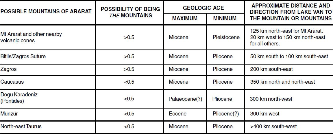
Table 6. Summary of the possible geologic age for the formation of the Mountains of Ararat.
The originally low-lying magmatic arcs of the Pontides (pre-Dogu Karadeniz Mountains) are not included in Table 6 because they were not uplifted until much later, and are therefore unlikely candidates for the Mountains of Ararat. If the Mountains of Ararat were part of the magmatic arcs of the Pontides, one could push the 150th day into the Mesozoic. However, the proximity of the Pontides to the Miocene ocean (Flood waters?) to the south would argue that the ground could not be described as dry until after deposition of Miocene marine sediments and recession of water. If Noah could look to the north and see the Black Sea, the ground would have always been covered with water and never dry. The combination of the distance the Pontides are from Lake Van and the east side of the Plain of Shinar, and their proximity to the Black Sea, make them poor candidates for the Mountains of Ararat.
The geological age of the mountains in and around Urartu indicate that the 150th day of the Flood should be placed somewhere between the Palaeocene and Early Pleistocene, depending on the identification of the true Mountains of Ararat. Since the year of the Flood lasted another seven months with significant geological activity (at least massive erosion due to receding Flood waters), the Flood/post-Flood boundary must be well after the Palaeocene. The biblical requirement for dry ground (Genesis 8:13, 14) would make the likely location for the boundary sometime after the marine regression in the Early Pliocene. The most likely place for the Flood/post-Flood boundary, based on the geologic age of the more probable Mountains of Ararat and the biblical requirement for nearby dry ground, is late in or after the Pliocene.
To place the Flood/post-Flood boundary earlier in the geologic column, it could be argued that the true Mountains of Ararat were formed in the Palaeozoic or Mesozoic but did not survive post-Flood events. One difficulty with the argument is reconciling it to the biblical account (Genesis 8:13, 14) that the Mountains of Ararat survived until the ground was dry. The geologic history of Urartu is dominated by marine sedimentation from the Palaeozoic through the Mesozoic and into the Miocene. In addition, this scenario would then require the Mountains of Ararat to survive into the Miocene and subsequently erode, while all listed Cainozoic mountains survive. Such selective catastrophism seems unlikely.
Global Sea Level Changes
Changes in the sea level on a global scale are called eustatic changes. These changes affect every continent simultaneously and are in addition to any local, regional, or single-continent changes. From the account in Scripture, one should expect the worldwide Genesis Flood to include tremendous eustatic changes and these changes should be recorded in Earth’s sediments. After the Flood there should be a limit to eustatic changes as constrained by the places where Noah and his family lived. Scripture also indicates that after the Flood there was a bound set on the sea that it should not pass. Investigating global sea level changes in light of Scripture should give clues to location of the Flood/ post-Flood boundary.
Sea level estimates are generally based on:
- (1) interpreting the presence of fossils of marine creatures and plants as an indication the area was covered by sea, and interpreting the presence of fossils of terrestrial creatures and plants as an indication that the area was land; or
- (2) interpreting trans-gressions and regressions of the sea, as shown by sequence stratigraphy, as eustatic changes; or
- (3) a combination of both.
From a Flood-model view, it is difficult to say when water was not covering an area based on terrestrial fossil content. However, it is safe to say that if marine fossils are present, the area was covered by water. Transgressions and regressions may be indicative of the direction of water and sediment flow, rather than the actual water level. However, transgressions and regressions still indicate the sea level had to be at least at the indicated height in order to move, erode, and deposit sediment.
There are three widely cited eustatic studies —Vail, Mitchum and Thompson in 1977,210 a subsequent refinement by Haq, Hardenbol and Vail in 1987,211 and the study by Hallam in 1984.212 The eustatic curve and its subsequent refinement by Vail et al. is commonly referred to as the ‘Vail curve’, and is based on seismic stratigraphy. Data supporting the Vail curve has only been published for the Mesozoic and Cainozoic portions;213 however, the Palaeozoic portion resembles that of Sloss.214 Others report similar findings for the Palaeozoic.215,216 The Hallam curve is based on hypsometric analysis and area-elevation data of marine deposits from palaeogeographic atlases. The Vail curve provides detailed eustatic data through the Holocene, whereas the Hallam curve shows only general trends and ends with the Pleistocene.
Striking differences in the two curves are the heights of the Late Cretaceous and mid-Ordovician maximums, and the absence of large rapid sea level changes in the Hallam curve (see Figures 7 and 8). The true height of the mid- Ordovician maximum sea level is difficult to establish accurately because of the variations in continental palaeohypsometries and isostatic adjustments between then and now. According to a recent analysis of 13 Palaeozoic landmasses’ flooding records and palaeo-hypsometries, the Hallam mid-Ordovician maximum is substantially lower and closer to the mid-Cretaceous maximum. The rapid sea level changes are not present in the Hallam curve because the analysis method does not have the time resolution and global correlation, at least at the present, to indicate such rapid changes. Nevertheless, the major trends of the Vail and Hallam curves are in good general agreement.
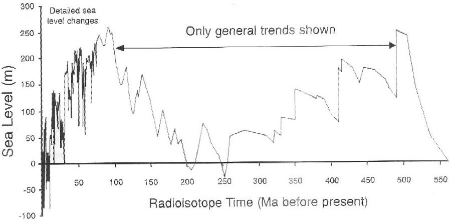
Figure 7. Global changes in sea level (after Vail et al.)
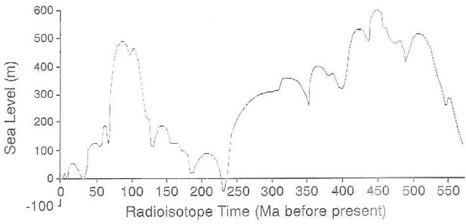
Figure 8. Global changes in sea level (after Hallam).
Quaternary eustasy is an area of great debate and uncertainty among evolutionary researchers, as Oard and others have documented.217,218,219 However, what is agreed upon is a large rise in sea level after the Ice Age, and a eustatic sea level of -8 to -12 m at 7,000 radioisotope years ago.220 Therefore, for the present discussion, the most recent rise in sea level, at the end of the Pleistocene in Vail’s curve, will be associated with the end of the post-Flood Ice Age.
Studies of many areas appear to be confirming Vail’s general curve, including what appears to be large and rapid variations in the sea level throughout the Phanerozoic. The accuracy in timing and magnitude of Vail’s sea level changes has been questioned,221 but the major trends are generally accepted (that is, first and perhaps second order eustatic changes). The global application of third-order and higherorder sea level variations (that is, detailed variations in the 1 to 3 Ma radioisotope time-frame) remain the topic of much research and discussion. (Could it be that global third-order sea level changes correspond to daily tides during the Flood?) A recent review of sequence stratigraphy suggests potential application to creation models;222 however, the significance of the eustatic curve is not addressed.
The general agreement between the Vail and Hallam eustatic curves, based on independent data and different methods of analysis, demonstrate the first-order trends in sediment character are real. Both eustatic curves indicate two major peaks in the sea level during the Phanerozoic. These peaks are in the Late Ordovician and the Late Cretaceous, and they are separated by an apparent low sea level in the Late Permian to Early Jurassic.
After the Cretaceous the sea level decreases, but the behaviour is not monotonic. The curve from Hallam shows a dramatic drop in the sea level at the end of the Cretaceous, and again at the end of the Eocene, with significant, though smaller, variations in the Miocene, Pliocene and Pleistocene. In contrast, the Vail curve223 shows a tremendous drop (>250 m) in the mid- Oligocene, a large surge (125 m) and drop (250 m) in the Miocene, and significant variations (up to ±85 m) until the Holocene (see Figure 9).
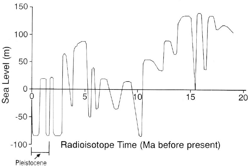
Figure 9. Details of the global changes in sea level (after Vail et al.)
Scripture: Dry Ground and a Bound to the Sea
Eustatic curves must be interpreted in light of the biblical account to determine the Flood/post-Flood boundary.Genesis 8:13–14 alludes to a stable sea level late in the year of the Flood. On the 314th day of the Flood, Noah observed that the ‘face of the ground was dry’ (verse 13). The following verse records that ‘the earth was dried’. After the Flood, God stated that he would never again destroy the earth with a Flood (Genesis 8:21–22; 9:11–16 and Isaiah 54:9).
In Job 26:10, Psalm 104:9, and Jeremiah 5:22, God states He had set a bound to the sea that it should not pass:–
‘He hath compassed the waters with bounds, until the day and night come to an end.’ Job 26:10 (KJV)
‘Thou coveredst it with the deep as with a garment: the waters stood above the mountains. At thy rebuke they fled; at the voice of thy thunder they hasted away. They go up by the mountains; they go down by the valleys unto the place which thou hast founded for them. Thou has set a bound that they may not pass over; that they turn not again to cover the earth.’ Psalm 104:6–9 (KJV)
‘Fear ye not me? saith the Lord: will ye not tremble at my presence, which have placed the sand for the bound of the sea by a perpetual decree, that it cannot pass it: and though the waves thereof toss themselves, yet can they not prevail; though they roar, yet can they not pass over it?’ Jeremiah 5:22 (KJV)
Job 26:10 and Jeremiah 5:22 are speaking of God’s greatness and use the boundary of the sea as a real life example. Psalm 104:6–9 is speaking about the Flood and the boundary of the sea at the end of the Flood. In each case the boundary is spoken of as something permanent and applicable to all time since the Flood. The Scripture, taken straightforwardly, is saying the bound of the sea has not been transgressed since the Flood.
The Scripture indicates the sea level was at the bound of the sea during the time of David (author of Psalm 104) and Jeremiah. The level of the sea has changed little between the time of David and Jeremiah, and today, therefore the present sea level is at or near the boundary of the sea. It follows that the post-Flood sea level has not been much higher, if any, than it is today.
Taking these Scriptures straightforwardly means the global sedimentary record should show a major decreasing trend in the sea level during the late stages of the Flood. At some point the sea level will reach the present level and never rise higher again. The sea level could go lower during the Ice Age but would not rise above the bound to the sea. This suggests a placement of the Flood/post-Flood after the mid-Pleistocene boundary using Vail’s curve, and after the Pliocene using the less detailed Hallam curve.
Eustasy and Biblical Lands
There are three places or areas mentioned in Scripture that give clues to the Flood/post-Flood boundary. These places are where Noah and his descendants lived at or travelled through immediately, or soon, after the Flood. In sequential order they are:–
- (1) in or near the Mountains of Ararat (Genesis 8:4, 15–22; 9:1–22),
- (2) the area east of the plain in the land of Shinar (Genesis 11:2), and
- (3) the plain in the land of Shinar (Genesis 11:2–6).
The geology of these areas should give some insight to the location of the Flood/post-Flood boundary in the geologic column. For brevity, the plain in the land of Shinar will be called the Plain of Shinar.
Scripture says the ground was dry on the 314th day of the Flood, Noah left the Ark on the 371st day, and shortly thereafter Noah planted a vineyard. The land around the Mountains of Ararat is the ancient land of Urartu. The geologic evidence indicates the land of Urartu was dominated through the Early Miocene by marine facies. Regional uplift of eastern Anatolia began in the Middle Miocene and was completed in the Early Pliocene.224 Uplift of the entire Anatolian-Persian Plateau also appears to have been completed by the Early Pliocene; this is indicated by a regional unconformity in the Early Pliocene in the Silvas Basin (in central Turkey) and in far eastern Turkey.225 The ground in Urartu could not be dry until after the Miocene, which is in agreement with the eustatic curves. The earliest Noah could have planted a vineyard would have been after the Miocene. This places the Flood/post-Flood boundary after the Miocene.
Travelling out of the east and coming to the Plain of Shinar, Noah and his descendants would have to travel through the Zagros Mountains. The area of the Zagros Mountains was dominated with marine sediments through the Miocene, after which the formation of the mountains began.226,227,228 To come out of or even cross the Zagros requires Noah and his family to approach the Plain of Shinar sometime after the Miocene and perhaps after the Pliocene.
The Plain of Shinar would have to be land (as opposed to sea, lake or swamp), and therefore above the post-Flood eustatic level, to reasonably be called a plain. The Plain of Shinar is in the region called Mesopotamia, which in Greek means ‘between two rivers’. The oldest identifiable inhabitants of the Plain of Shinar are the Sumerians; ‘the old west Semite form of the name (Sumer) appears to have been Shinar’.229 The Sumerians lived in southern Mesopotamia, so ‘properly speaking, Sumer was the territory from modern Baghdad south to the Persian Gulf.’230 Over this entire distance the elevation increases by about 37 m.231
The geology south of Baghdad is dominated by marine facies through the Miocene, with fluviatile gravels, sands and muds in the Pliocene and Pleistocene.232,233,234 A reasonably dry plain would not be possible until after deposition of the Miocene marine sediments, and probably after deposition of the Pliocene sediments. These sediments suggest the Flood/post-Flood boundary is in the Pliocene or Pleistocene.
A post-Flood sea level above the present level would flood a tremendous portion, if not all, of the plain turning it into an extension of the Persian Gulf. The Plain of Shinar rises to an elevation of only 37 m at Baghdad. The post- Flood sea level would be limited to near the present level for God’s promises about not sending another flood to have meaning Noah and his immediate descendants residing in the low-lying Plain of Shinar. According to Hallam’s curve the Plain of Shinar would not be dry until after the Pliocene. According to Vail’s curve the Plain of Shinar would not be dry until after the mid-Pleistocene.
Scripture mentions human activity right after the Flood in three places. The marine facies in these areas indicate this activity could not have occurred before the Early Pliocene and probably not until the mid-Pleistocene. This suggests the Flood/post-Flood boundary would have to be somewhere in the Pleistocene.
Post-Flood Isostatic Adjustments and the Ice Age
Post-Flood isostatic and eustatic adjustments are expected in some post-Flood models.235,236,237 However, these adjustments would result in a lowering of the sea level; the probable mechanism being subsidence of the ocean floor from thermal cooling, or a rising of continents from isostatic adjustments. Both have the same effect of lowering the sea level, and therefore the sea would not transgress the bound God placed at the end of the Flood. The Ice Age is generally expected to cause a drop in the sea level followed by a rise, all of which should remain within God’s ordained bound to the sea.
Oard has suggested an eustatic level 40 m above the present sea level at the end of the Flood, which is then followed by a eustatic decrease to roughly 60 m below the present level at Ice Age maximum.238 He estimates there is an equivalent of about 60 m of water stored in the Antarctic and Greenland ice sheets, which if melted would only produce an eustatic rise of 40 m due to isostatic adjustment. If Oard’s eustatic model is correct, the Flood/post-Flood boundary would be after the Miocene according to Hallam’s curve, and in the Early to mid-Pleistocene according to Vail’s curve.
A eustatic level immediately after the Flood of a few tens of metres above the present level would produce dramatic changes in the Middle East, particularly in the Plain of Shinar. This seems to go against one’s first impression when reading Genesis 8:21–22; 9:11–16, Isaiah 54:9, Job 26:10, Jeremiah 5:22, and Psalm 104:6–9. Oard’s eustatic model would predict that the Plain of Shinar would be very wet and not a plain until several hundred years after the Flood.
The difference between Scripture and Oard’s model (or any other model) for eustatic change during the Ice Age may be clues to understanding post-Flood isostatic adjustments in the Earth’s crust, or the distribution of water within Earth’s reservoirs. This could include variation in the elevation of mid-ocean ridges, and/or tectonic and isostatic movements of continents. Alternately, these differences could be resolved by considering the total amount of Flood waters retained on the continents:–
- (1) in extinct lakes and rivers, for example, Hopi, Grand, Vernal, Bonneville, Lahontan and Missoula Lakes, and the like on other continents,
- (2) in an increased size of present inland seas, lakes and rivers, for example, Caspian Sea, Aral Sea, Black Sea, Dead Sea, etc., and
- (3) in ground water, including what are now dry desert areas such as the Sahara, Gobi, the American south-west, etc.
As Scripture seems to indicate, it may be that the post- Flood eustatic level has always been at or below the present level of the sea. Water may have moved first from terrestrial locations (lakes, rivers and ground water) to Ice Age glaciers, and then to the present ice sheets on Greenland and Antarctica. Preliminary estimates indicate the largest unfilled storage capacity lies underground. It appears that there may be an adequate capacity to store water that resided in Ice Age glaciers in the ground.239
At the end of the Flood, all the Earth’s sediments would have been saturated with water. It would take time for the water to flow out of the saturated sediments and decrease continental groundwater storage to near the present level, assuming present precipitation rates. The increased precipitation in the post-Flood environment could have extended the saturated ground conditions to several centuries, approaching the time of the Ice Age maximum. This scenario avoids an end-of-Flood sea level above the present level, allows a post-Flood Ice Age decrease in sea level (if necessary) and subsequent increase in sea level, and conforms to the straightforward reading of Scripture. More research is needed in this area.
A Flood Model Perspective of Eustatic Curves
From a Flood-model perspective, the time between the two major eustatic peaks (in the Ordovician and the Cretaceous) was also during the Flood. Earlier placement of the boundary, at the end of the Palaeozoic for example, implies there was a second flood that was as large as, or nearly so, as that of the Genesis Flood. Placing the boundary at the end of the Mesozoic would end the Flood during a very high stand of water which covered most of the Earth. This does not fit the description of the end of the Genesis Flood.
The general decline of the sea level throughout the Cainozoic is reminiscent of the Flood waters receding off the land from the 150th to the 314th day of the Flood. This suggests that:
- (1) the 150th day of the Flood was at or after the eustatic peak in the Late Cretaceous, and
- (2) the Flood/post-Flood boundary is very late in the Cainozoic.
Some may be concerned by the variation in sea level during the Flood and the appearance of dry land in the middle of the first 150 days. One should not assume, a priori, from Genesis that the Flood waters:
- (1) instantly covered the Earth, or
- (2) increased and decreased in a monotonic manner over the entire surface of the Earth.
God did not state that all areas were simultaneously and continuously covered by water, while the waters prevailed on the Earth for 150 days.240 Some areas may have been repeatedly covered and uncovered by the Flood waters, while other areas may have been above water for weeks or months into the Flood. The ‘prevailing’ of waters for 150 days does not mean total covering, because it was forty days before the Ark was floating (Genesis 7:17–18), and the waters had to ‘prevail exceedingly’ to cover all the high hills, and later the mountains (Genesis 7:19–20).
God’s stated purpose for the Flood was to destroy man, fowls, and all creatures on dry land (Genesis 6:7, 17; 7:21–23). God did not say they were all to die instantly or only during the first 40 days. In addition, the occurrence of animal tracks and fossil preservation of soft parts241 throughout the geologic column suggests animals survived well into the Flood and had some land to walk on (as opposed to constantly swimming).
Global Sea Level Summary
When using Scripture to guide the interpretation of eustatic curves, the Flood/post-Flood boundary appears to be very late in the Cainozoic. If the Scripture’s statements about a bound to the sea can be taken straightforwardly, the Flood/post-Flood boundary would correspond to a sea level near where it is today. The high eustatic level through all but the last fraction of the Cainozoic, well above the present level, indicates God did not apply His boundary to the sea before the mid-Pleistocene. This places the Flood/post-Flood boundary after the mid-Pleistocene using the Quaternary eustatic curve of Vail.
Comparison of Scripture clues with marine sediments in the land of Urartu indicates the Flood/post-Flood boundary is after the Miocene. The geology of the Mountains of Ararat region and the Zagros Mountains (east of the Plain of Shinar) indicates the area was not above sea level until after the Miocene; the same observation is made for the Plain of Shinar. A more detailed review of the geology of these areas may be able to place tighter constraints on the Flood/post- Flood boundary.
Placing the Flood/post-Flood boundary at the end of the Mesozoic would end the Flood during a very high stand of water that meets the description of a near global flood rather than the end of the Flood. Placing the Flood/post-Flood boundary earlier in the geologic column, near the end of the Palaeozoic, implies there was a second worldwide flood that was as large as, or nearly so, as the Genesis Flood. Placement of the boundary at any place other than late in the Cainozoic, particularly before the mid to Late Pleistocene, requires a transgression of the bound God placed on the post-Flood sea and flooding of the Plain of Shinar.
Formation of Fossil Fuels
Fossil fuels provide several clues to the Flood/post-Flood boundary. If fossil fuels, in substantial quantities, can be produced only as a result of an enormous global catastrophe, then the source rock for these fossil fuels can only be Flood deposits. Conversely, fossil fuels could be indicative of post- Flood environments if the existing deposits are relatively easy to make and require only minor catastrophes. In addition, the length of time required to grow the raw organic materials necessary for making fossil fuels can give clues to identification of fossil fuels as either Flood or post-Flood deposits. The origin of fossil fuels, the total quantity and distribution by source rocks, as well as the nature of the source rocks give clues to the Flood/post-Flood boundary.
Source rocks are the rocks or strata that were the original sources for the fossil fuels, not the reservoirs in which the fuels currently reside. The source rock for coal is easy to establish because coal does not migrate. Identifying the source rocks for oil and natural gas are difficult to determine, but can be reasonably established.
Origin of Fossil Fuels
Coal, oil, and natural gas are usually thought of as fossil fuels, that is, they are the altered remains of buried marine and terrestrial life. The vast quantities of fossil fuel found in Phanerozoic deposits, which contain many other fossils, argues for a catastrophic burial of tremendous quantities of organisms as the origin of fossil fuels. However, the catastrophe could have occurred after the Flood, and perhaps even before the Flood for the minor amounts of Precambrian fossil fuels.
It is plausible that oil and gas were formed as the result of biological activity of deep-living micro-organisms. But, the relatively minor amounts of deep-living micro-organisms, discovered below a hundred metres or so, would be hard pressed to generate the world’s reservoirs of oil and gas in a short creationist time-frame. In addition, organisms that can generate or synthesise oil have not been discovered.
For hypothetical oil-producing deep-living organisms to generate the vast resources of oil and gas, an enormous quantity of carbon must be available. Consequently, even if oil could be produced by deep-living organisms, vast amounts of organic carbon must be buried in highly concentrated layers within sedimentary deposits. This requires a catastrophic burial of tremendous quantities of organisms.
There is room for an abiogenic origin of oil and gas within the creationist paradigm.242,243 This would mean fossil fuels were created by non-biological chemical reactions, or God created these fossil fuels. If oil and gas had an abiogenic origin, an explanation for tremendous quantities of vegetation and rapid biological formation of oil and gas would not be needed by creationists.244
The single attempt to find abiogenic oil and gas was a failure. A 6 km deep hole was drilled through granite in Sweden in search of oil and gas. None was found.245 In contrast, an analysis of the plausible capacity of the pre- Flood biosphere shows it could easily have supplied all the organic carbon required to form fossil fuels.246 There is little reason to believe oil and gas have an abiogenic origin, and good evidence for their biogenic origin.
Coal
Coal is plant matter that has been altered under an oxygen free and high temperature environment. Many coals contain wood cell structures, leaves, bark, twigs, logs, and tree trunks. Carboniferous coals consist of tree ferns, lycopods, and some gymnosperms, whereas Cretaceous and Eocene coals consist mainly of gymnosperms and angiosperms.247 This change in tree types that make up coals may reflect the differing times it took to waterlog and sink various types of trees and vegetation,248 or ecological zonation, or both. Those who place the Flood/post-Flood boundary in the Mesozoic or earlier might interpret this as a change in the dominant type of trees living before and after the Flood.
Until the last three decades, creationist researchers thought that coal beds were a direct result of the Flood. For over 200 years creationist scientists maintained that coal resulted from enormous mats of rafting vegetation that sank in the Flood waters and were subsequently covered and altered. This has been pointed out by many geologists last century,249 creationists earlier this century,250,251,252,253 and more recently by others.254,255,256,257,258 In the last three decades some researchers have suggested a Late Palaeozoic to Late Mesozoic placement of the Flood/post-Flood boundary.259,260,261,262 This would require many coal beds to be deposited after the Flood.
Oil (Petroleum)
Oil is generally thought to be produced from plant and/ or animal remains under conditions similar to those required for coal. Some of the main reasons for believing oil has a biogenic origin are as follows:
‘Crude oil can also contain a small amount of various decay-resistant organic remains, such as siliceous skeletal fragments, wood, spores, resins, coal and lignite, and many other remnants of former life.
- 1. Petroleum commonly is associated with sedimentary rocks, principally those deposited under marine conditions but also including continental sediments: conversely, there is a complete absence of commercial deposits of petroleum where only igneous or metamorphic rocks (formed under great heat and pressure) are present.
- 2. Petroleum exhibits a particular optical activity (the ability to rotate the plane of polarized light) associated almost exclusively with compounds of biogenic origin.
- 3. Most types of petroleum contain complex hydrocarbon compounds termed porphyrins, formed either from the green colouring matter of plants (chlorophyll) or from the red colouring matter of blood (hemin).
- 4. Carbon isotope ratios (13C/12C) indicate that petroleum may be derived in large part from the lipid (fats and waxes) fraction of organisms.
- 5. Many petroleum-like hydrocarbons have been found in recent marine sediments as well as in soils in many places throughout the world; these occurrences form a link between present living organisms and the petroleum found in sediments of older geologic ages.
The organic material that is the source of most petroleum has probably been derived from the singlecelled planktonic (free-floating) plants, such as diatoms and blue-green algae, and single-celled planktonic animals, such as foraminifera, that live in the aquatic environments of marine water, brackish water, or fresh water.’263
Oil shale appears to have a similar origin:–
‘Some oil shale kerogens are composed almost entirely of algal remains, whereas others are a mixture of amorphous organic matter with a variable content of identifiable organic remnants. The main algal types are Botryococcus and Tasmanites.’264
Today Botryococcus is fresh or brackish water algae and Tasmanites is marine algae.
In 1980 oil was found forming in the Guaymas Basin (a 6,500 feet/1,980 m deep trench in the Gulf of California) in association with hydrothermal vents. Researchers now estimate a total 4 x 10¹³ g of oil in the 30 km2 area around the active vents.265 The organic source for the oil was found to be the surrounding sediment, which is described as diatomaceous ooze with some terrestrial silty mud. The diatomaceous ooze is estimated at about 400 m thick. This finding supports the idea that marine algae (diatoms and the like) were the primary source for oil.
Oil does not appear to be forming in significant quantities today. The quantity of oil forming in the Guaymas Basin is four orders of magnitude smaller than the known oil resources, and is therefore insignificant. The potential for post-Flood oil production in the ocean could be great if all hydrothermal vents were as productive as those in the Guaymas Basin. However, the failure thus far to find oil forming at other hydrothermal vents along the Pacific and Atlantic mid-ocean ridges severely limits the amount of post- Flood oil that could be forming.
Natural Gas
The origin of natural gas has been more of a mystery to scientists, although thermal decomposition of oil has been the favourite theory. Natural gas is found in association with both coal and oil, and is therefore believed to be the by-product of both.
‘Many of the source rocks for significant gas deposits appear to be associated with the worldwide occurrence of Upper Palaeozoic coal.’266
For example, the Groingen gas field of the Netherlands with more than 1.7 x 10¹²m3 of reserves in Permian rock is above deeply buried Carboniferous coal. Thus volatiles in coal may be the raw material for generation of gas in these occurrences.
Experiments investigating the origin of natural gas from oil have provided low yields of methane (<50 per cent) at temperatures between 580 and 700°C, whereas natural gas is typically between 70 and 100 per cent methane. Recent experiments indicate that natural gas may be a result of catalytic conversion of oil that takes place at mild temperatures (200°C) in source rocks.267,268 In these experiments the source rock was fine-grained carbonaceous sedimentary rock. Unlike prior experiments, these experiments used natural rock as the catalyst and produced methane in concentrations similar to natural gas. It is interesting that the addition of a moderate amount of water (2.4 wt% rock), but not too much, increased the catalytic activity and conversion selectivity to methane.
Gas could be forming today in significant quantities by continued catalytic reactions. Even so, its present formation does not alter the important burial and formation of the original raw materials, since gas appears to be the by-product of oil or volatiles in coal.
Fossil Fuel Origin Summary
The geologic, chemical, and experimental evidence strongly supports the biogenic theory for the origin of fossil fuels. Therefore the organic carbon making up the vast fossil fuel resources must have been deposited during the Flood or post-Flood catastrophes. The experimental evidence also indicates that coal, oil, and gas require very little time to form.269,270 However, the formation time is so short that one cannot distinguish between fossil fuel formed during the Flood or shortly thereafter.
Global Inventory of Fossil Fuels
The estimated geologic resources of each fossil fuel is shown in Table 7. These estimates include proved, indicated, inferred, and undiscovered resources. This means a fair amount of educated guess-work is involved, particularly for undiscovered resources. The estimates of geologic resources change through the years as a result of new data or different assessments of proved, indicated, inferred, and/or undiscovered resources. The estimates in Table 7 are rounded to two significant digits because of the uncertainty involved, even though some authors cite several digits of precision.
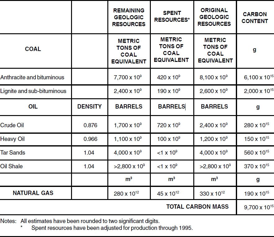
Table 7. Estimated geologic resources of fossil fuels.
Geologic resources are much larger than the reserves usually cited. (The term reserves is usually applied to technically and economically recoverable resources using available technology. The term resources is applied to all the fossil fuel deposits that theoretically could be recovered independent of cost or technology limitations.) In the case of coal, geologic resources are more than an order of magnitude larger than recoverable resources. For oil and natural gas, geologic resources may be two to five times larger than recoverable resources.
The total geologic resources of coal listed in Table 7 are from the World Energy Conference (WEC) Survey of Energy Resources 1980,271 and are in excellent agreement with Bois et al.272 and comparable to those of Riva.273 The estimated spent resources of coal is my estimation based on data from Rotty,274 Rotty and Marland,275 and the Energy Information Administration (US).276
The WEC data is in metric tons of coal equivalent, where one coal equivalent has a heating value of 7,000 calories per kilogram. The average heating value of anthracite and bituminous coal might be 20 per cent more than 7,000 calories per kilogram, and that of lignite and sub-bituminous coal roughly 20 per cent less. The masses of coals listed in the table have not been adjusted by these factors and are as given by the WEC.
The estimated geologic resources and spent resources of crude oil are from Masters et al.,277 as cited by the Energy Information Administration (US).278 Masters et al. estimated the geologic resources at a little more than twice that estimated by Bois et al., slightly larger than that cited by Klemme and Ulmishek, but comparable to that of Riva and a number of different estimates cited by Tissot and Welte.279 Some estimate the geologic resources of crude oil may be as high as twice that estimated by Masters et al., at 4 trillion barrels.280
The estimated geologic resources of heavy oil and shale oil are calculated from Riva’s recoverable resources and recovery rates. The recovery rates are assumed to be at 60 per cent and 37.5 per cent for heavy oil and shale oil respectively, as Riva suggests. The estimated geologic resources of tar sands are compiled from a number of authors as cited by the National Research Council (US)281 and are comparable to the estimate of Riva. The amount of spent resources of tar sands and shale oil are minimal because of their higher cost of refining.
The estimated geologic resources and spent resources of natural gas are from Masters et al., as cited by the Energy Information Administration (US). This estimate is five times greater than that of Bois et al., and nearly twice the size of some of the recoverable resource estimates cited by Tissot and Welte or the estimate of Riva.
The carbon content estimation of fossil fuels is based on the conversions used by Rotty and Marland.282 The carbon in coal is estimated at 74.6 per cent, by weight, for coal equivalent units. For oil the carbon content is estimated at 85 per cent by weight. The carbon content of natural gas is estimated at 574 g/m3.
A casual glance at Table 7 indicates there is a tremendous amount of fossil fuels on the Earth. The total quantity of geologic resources are important, because there is only so much organic material that can be grown, buried, and transformed into fossil fuels after the Flood. To put limits on the Flood/post-Flood boundary the distribution of these fossil fuels in the geologic column is needed.
The Distribution of Fossil Fuels in the Geologic Column
The distribution of original resources of oil and gas (that is, prior to loss by erosion, leakage, migration, etc.) by original source rock is shown in Figure 10. The data is based on the work of Klemme and Ulmishek.283 Also in Figure 10 are the reserves of coal according to the WEC Survey of Energy Resources (1980).284 The loss of oil and gas, estimated according to source rock area by Klemme and Ulmishek, is less than 2 per cent after the mid- Jurassic (Tournaisian), 3.2 per cent for the Upper Devonian through the mid-Jurassic, and 11.7 per cent for the Silurian. This represents a loss of less than six per cent of the original resources, assuming area lost is proportional to mass lost.
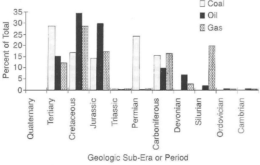
Figure 10. Distribution of source rock for coal, oil, and gas (after WEC and Klemme and Ulmishek).
A similar distribution of existing reserves of coal and oil, by original source rock based on the data of Bois et al. , is shown in Figure 11.285 Bois et al. give estimates of the distribution of natural gas by reservoir rock, not source rock; therefore their data for natural gas is not shown in Figure 11. Also shown in Figure 11 are the reserves of heavy oil and tar sands, according to Demaison.286 Bois et al. include some tar sands, so there is some overlap in the data. It is notable that there are no significant hydrocarbon source rocks known in Pleistocene or Holocene layers according to Klemme and Ulmishek, and Bois et al. , as well as others.
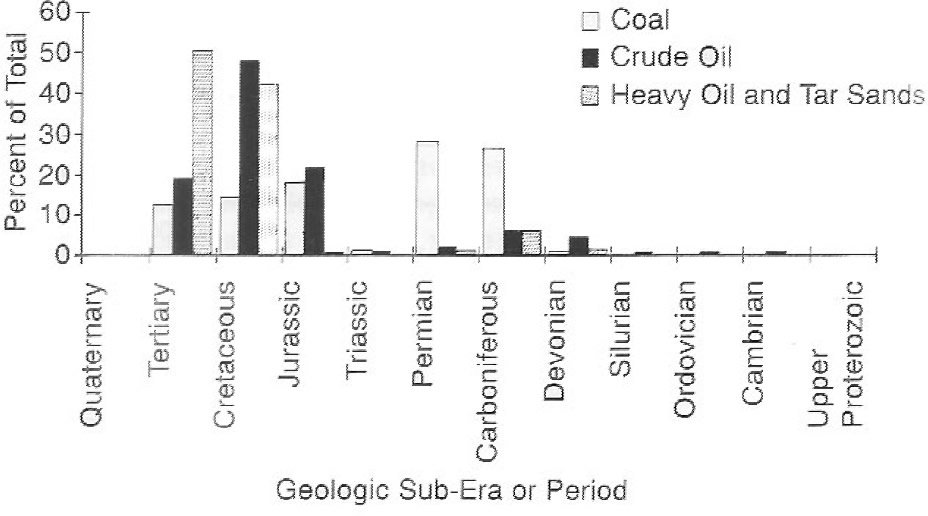
Figure 11. Distribution of source rock of coal, crude oil, and heavy oil and tar sands (AFter Bois et al. and Demaison).
The distributions by source rocks for Figures 10 and 11 are summarised in Table 8. A linear interpolation has been used to give distributions by era and periods in Table 8, and in Figures 10 and 11, where the data was not presented by era or period. As a result the actual distribution may be slightly different from that shown. This interpolation is expected to introduce a small amount of error in the table and figures. The error, which is probably less than a few per cent between periods, is less than the difference between the various estimates and the uncertainty in world geologic resource estimates.
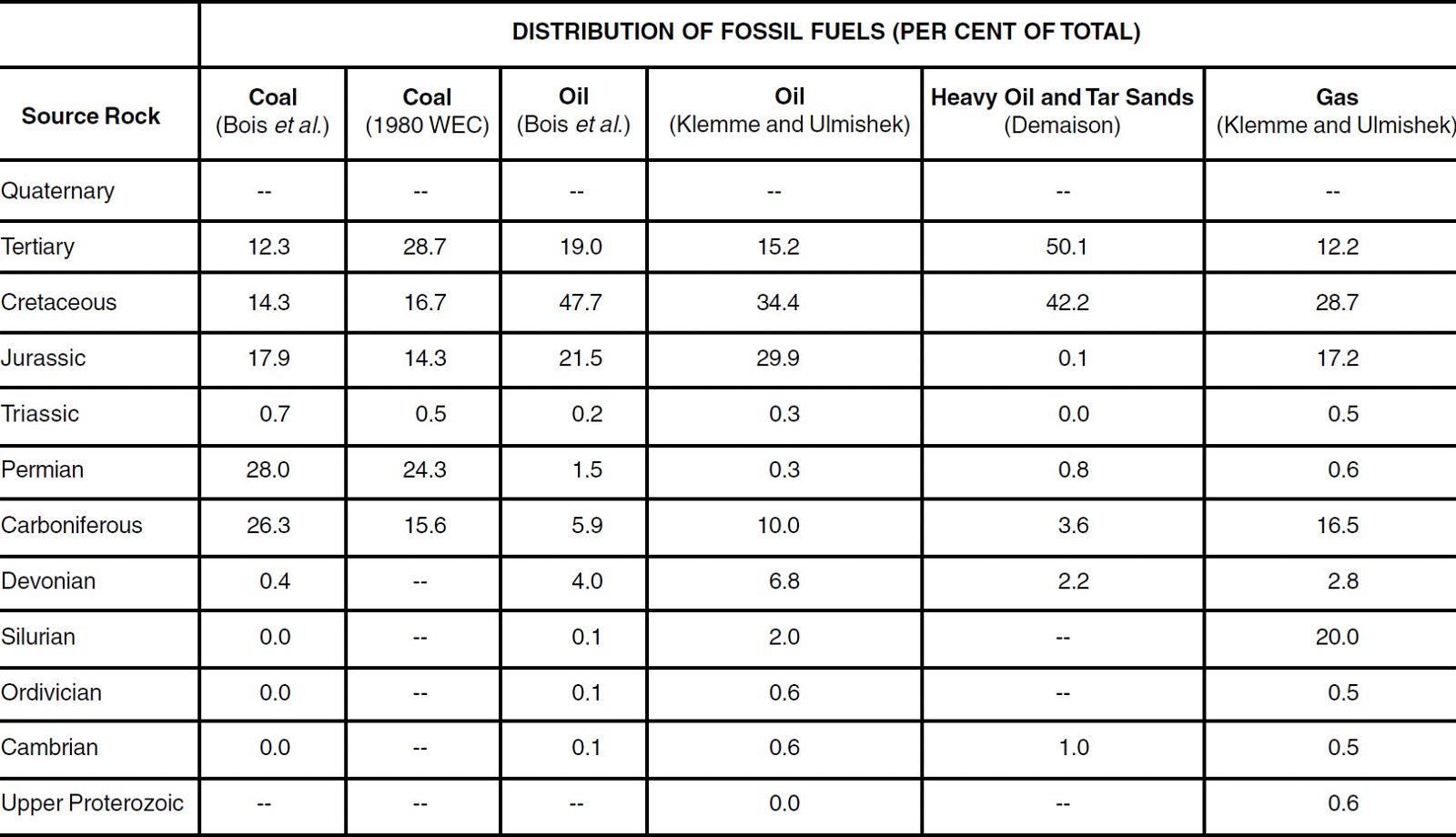
Table 8. Distribution of fossil fuel by source rock. Same data as in Figures 10 and 11.
There is a significant contrast between the estimates of Bois et al. and the WEC survey for coal, and between Klemme and Ulmishek and Bois et al. for oil. The differences may be due to discoveries of new coal and oil fields, and/or better estimations of known oil and coal source rock volumes. For coal, the WEC estimation was published in 1980 and the work of Bois et al. was published only two years later in 1982. The reason for the significant difference is not clear. For oil, the work of Bois et al. was published in 1982, whereas the work of Klemme and Ulmishek was published about a decade later in 1991. There have been significant changes in fossil fuel reserve estimations during this period of time.287
Independent of the absolute accuracy of the estimates, both indicate substantial amounts of coal, oil, and gas have Tertiary and Mesozoic deposits as their source rock. There is a limit to how much of these fossil fuels can be biologically grown, buried, and transformed in the time since the Flood.
Amazingly, between 12.3 per cent and 28.7 per cent of the coal resources are Tertiary in age, and between 31.5 per cent and 32.9 per cent are Mesozoic in age. For crude oil, between 15.2 per cent and 19 per cent comes from Tertiary source rock, and between 64.6 per cent and 69.4 per cent comes from Mesozoic source rock. The source rock for the huge Middle East oil fields, that contain over half of the world’s crude oil reserves, are Jurassic and Cretaceous. Over half of the heavy oil and tar sands comes from Tertiary source rock, and an additional 42.2 per cent comes from Mesozoic source rock. For natural gas, 12.2 per cent comes from Tertiary source rock, and 46.4 per cent comes from Mesozoic source rock.
These data indicate the Palaeozoic may have about half, to less than half, of the coal resources and about 40 per cent of the natural gas source rock. About 20 per cent or less of the source rock for crude oil, and less than 8 per cent of the heavy oil and tar sands, would be Palaeozoic.
Placement of the Flood/post-Flood boundary at or near the end of the Palaeozoic would require post-Flood time to be more productive in generating fossil fuels than the Flood. Placement of the boundary at or near the end of the Mesozoic would require post-Flood time to be more productive than the Flood at producing heavy oil and tar sands. Post-Flood time is not generally considered a time when great reserves of fossil fuel could be generated.
Geographical Distribution of Fossil Fuels
Parrish et al. have produced a series of maps showing the global distribution of coal and evaporite deposits for seven stages in the Mesozoic and Cainozoic.288 Their maps show a significant variation in distribution with geologic layer through the Vindobonian (Middle Miocene), with coal deposits being on continental interiors as well as coastal regions.
A wide distribution of coal deposits is also reported by Drewry et al. for the Mesozoic and Cainozoic.289 In the Eocene and Palaeocene they show coal deposits at numerous inland locations, including the north-west and the south-east edges of the region of ancient Armenia (Mountains of Ararat region), and west of Hudson Bay where Ice Age glaciers would have rapidly formed.
Klemme and Ulmishek list 47 major productive basins containing petroleum-generating source rocks.290 Fifteen of the 47 basins have Mesozoic source rocks. These 15 basins are distributed among Asia, Europe, North and South America, and in the Middle East. Fourteen of the 47 basins have Oligocene-Miocene source rocks. These 14 basins are distributed among every continent, except Australia and Antarctica. Only 18 basins have source rocks in the Palaeozoic. Bois et al. have similar findings.291
Major Tertiary oil shale deposits are found in the Green River Basin in the corner of Wyoming, Utah, and Colorado.292 There is an estimated 420 billion barrels of recoverable oil in these deposits, with an in-place resource of about 1100 billion barrels.
Demaison estimated a global resource of 2,000 billion barrels of heavy oil and tar.293 About half of this reserve, 1050 billion barrels, is located in the single super-giant Orinoco oil belt in northern Venezuela. The Orinoco belt has Oligocene sands as the source rock. Other heavy oils with Tertiary source rock include the Pear Springs, Asphalt Ridge, Hill Creek, and Sunnyside deposits in Utah (USA). These Utah deposits have Eocene sands as the source rock and contain about 10 billion barrels of heavy oil and tar.
Freidman summarised the United States’ coal production for 1989, which totalled 981.8 million tons of coal.294 By geologic epoch, 30 per cent of the US production was Tertiary and 8 per cent was Cretaceous. Palaeozoic coal accounted for 42 per cent. Table 9 summarizes production data for a few states where Cainozoic or Mesozoic coals are mined.
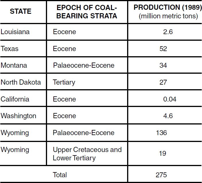
Table 9. A partial listing of United States coal production in 1989 from Cretaceous and Tertiary strata.
The lateral extent of some of the coal deposits is impressive. Western North Dakota, north-western South Dakota, eastern Montana, north-eastern Wyoming and southern Saskatchewan are underlain with huge Tertiary coal fields, in the Fort Union and Wastach Formations, that cover about 1.5 million km2. These areas are called the Powder River Basin and Northern Great Plains Region.
The coal seam in the Fort Union Formation is thick, exceeding 30 m in places. The vegetation pile that was transformed into this coal seam may have been between 150 and 300 m thick. This is not a trivial amount of vegetation.
These data illustrate the wide distribution of Cainozoic and Tertiary fossil fuels. The wide distribution of fossil fuels requires a large catastrophic event(s) to gather the raw organic material, allow it to deposit in thick layers, and subsequently bury it with sediment. The Flood could be expected to perform such catastrophism on a massive scale, but it is not clear that this could be accomplished in a plausible post-Flood environment.
Burial of Fossil Fuels
The source rocks for fossil fuels, like the vast majority of all Phanerozoic sedimentary rocks, appear to have been water deposited. The lack of soils below coal seams, the fine deposition line marking the bottoms and tops of the seams, the prevalence of underclays without roots or containing only broken root fragments, the presence of tree trunks without extended root systems, and the absence of significant mud/dirt, sand, and rock mixed in coal are all evidences of rapid deposition. Similarly, oil shales also appear to be the result of rapid deposition.
Source rocks for fossil fuels are found covering vast areas stretching thousands and even millions of square kilometres. The catastrophic event or events that produced such widespread deposits had to be enormous, dramatically affecting major portions of entire continents. However, only a limited amount of sediment could have been moved and deposited after the Flood.
If one assumes that the continental sediment deposition is proportional to marine sediment deposition after the Flood, the maximum post-Flood continental sediment can be estimated. The prior section on global sediment and erosion found a maximum limit of 1.2 x 10²¹ g of sediment could have been carried to the oceans after the Flood. This was about one twentieth of the continental sediment of 7.1 x 10²¹ g, of which 0.94 x 10²¹ is glacial sediment according to Hay.295 In comparison, Hay estimated the total continental Quaternary sediment at 13.57 x 10²¹ g. Assuming continental sediment deposition is proportional to marine sediment deposition, the maximum post-Flood continental sediment is 6.8 x 10²⁰ g.
At a density of 2.3 g/cm3, 6.8 x 10²⁰ g of sediment represent a maximum thickness of 2 m if spread uniformly over the present continents. This small amount of sediment is insignificant compared to the mass of sediment in which fossil fuels are buried. The burial of fossil fuels becomes more difficult when one estimates the mass of overburden that was originally in place and has been removed by subsequent erosion.
Time Required to Grow Raw Materials for Fossil Fuels
Gross primary production denotes the amount of carbon photosynthesized by plants. For the terrestrial biota much of the gross primary production is returned to the atmosphere by plant respiration and decay, reducing the acquired carbon to a lower level called net primary production. For marine biota the gross primary production is reduced by the amount of carbon dissolved and returned to the ocean reservoir, rather than the atmosphere. The net primary production is the amount of carbon captured and retained by all plants through photosynthesis, that is, the total increase less all losses. By comparing the net primary production with the amount of carbon in fossil fuels, biota, and soil detritus one can get a rough estimate of the time required to grow the organic raw materials. The following estimations are made assuming volcanic activity did not dramatically reduce sunlight photosynthesis, and thus limited the net primary productivity of the Earth.
In a steady state condition the average net primary production is zero, that is, all carbon acquired by growing plants is lost by destruction (fires) and decay. The average net primary production can be greater than zero by the continued growth of plants, principally trees, and/or an accumulation of carbon in reservoirs. Natural reservoirs include the formation of peat, accumulation of plant debris in swamps, and catastrophes that bury and retain biogenic matter. The present estimate of carbon accumulation in peatlands and wetlands is a meagre 0.14 x 10¹⁵ g of carbon per year.296
A recent estimate placed the terrestrial annual gross primary production at 180 x 1015 g of carbon, with forests being the largest contributor.297 This is about twice as large as earlier estimates.298,299 A recent estimate places the terrestrial net primary production at 53.2 x 10¹⁵ g of carbon, or 29.6 per cent of the gross primary production.300 This estimate for the net primary production is comparable to earlier estimates of 38 to 78 x 1015 g of carbon.301,302
Presumably the large net primary production during the present time is caused by new vegetation refilling cleared or deforested areas and enhanced growth promoted by the increase in atmospheric CO2. Observations at New Zealand and at Mt Shasta, California, suggest that rapid new growth will give a peak of net primary production during the first 300 to 500 years (under present weather conditions).303 By about 1200 to 7000 years (in radioisotope time) an originally barren area will have approached equilibrium. Experiments have found that plants’ growth response to a doubling in CO2 is between 24 and 50 per cent.304
At a net primary production of 53.2 x 10¹⁵ g of carbon per year, it would take about 181 years of terrestrial growth to accumulate the total amount of carbon retained in all fossil fuels. It would also take only 12 years of terrestrial growth to accumulate the total amount of carbon retained in the pre-industrial terrestrial biota (600 x 1015 g carbon).305 An additional 30 years of terrestrial growth is all that would be needed to generate the carbon content of plant detritus in soil (1,560 x 1015 g carbon).306 It seems incredible that it would take only 233 years, at current net primary production rates, to accumulate in terrestrial plants the carbon in all the existent fossil fuels and terrestrial biota.
The annual net primary production of the oceans has been estimated at 12 to 25 x 1015 g of carbon.307,308,309 More recently, the net primary production of the oceans has been estimated at 3.4 to 8.3 x 10¹⁵ g of carbon per year.310 The ocean, which covers 71 per cent of the Earth, has a low productivity compared to the land.
Since oil appears to have a predominantly marine origin, one should consider how long it would take for marine plankton to accumulate the amount of carbon stored in oil. Assuming a mid-range estimate for the net primary production of 10 x 1015 g of carbon per year it would only take 138 years. The dry matter biomass of the ocean is estimated at 3 x 10¹⁵ g.311 If the marine biomass (dry weight) is about 45 per cent carbon, as estimated by Sharp,312 it would take just a few months to accumulate the amount of carbon retained in all the marine biota. Only 138 years would be required to accumulate all the carbon retained in the world’s oil and ocean biota. If the higher estimates of net primary production are used, the accumulation time would be substantially less. Like the terrestrial considerations, it seems incredible that this much carbon could be accumulated in such a short period of time.
Even so, there is a tremendous difference between
- (1) accumulating this much carbon after the Flood, and
- (2) uprooting forests and other biota, rafting much of the biota together to deposit at various and scattered locations, and finally burying the organic material under and throughout significant layers of post-Flood sediments.
This description of hydraulic activity is more reminiscent of a global Flood than of post-Flood times. A cataclysmic event large enough to bury much of the Tertiary organic carbon would be near global in extent and require a major transgression of the bound God placed on the seas.
Admittedly the above estimates are rough, but they show that it is plausible for sufficient growth to occur after the Flood, to account for the carbon in all Phanerozoic fossil fuels. However, the estimates have
- (1) assumed a 100 per cent burial and conversion to fossil fuel efficiency, and
- (2) ignored the amount of biogenic carbon in sediments that are not part of the fossil fuel resources.
One would expect, during the Flood and post-Flood catastrophes, that a major portion of the vegetation would be scattered throughout the sediments and some would rot and decay. If the burial and conversion efficiency was 10 to 15 per cent, which seems high, 1,500 years would be needed to accumulate the carbon, and some additional time would be needed for catastrophes to produce all the fossil fuel deposits.
Budyko, Ronov and Yanshin estimate 7.8 x 10²¹ g of organic carbon (non-carbonate) in Phanerozoic sediments, excluding the Quaternary.313 This is 810 times the amount stored in geologic resources as cited in Table 7, or about 0.34 per cent of the total mass of Phanerozoic sediments. About 127,000 years would be required to accumulate this much carbon at the current net primary production rate. (They estimate an additional 49.4 x 10²¹ g of carbon are stored in carbonates throughout the Phanerozoic sediments, excluding the Quaternary.)
The amount of organic carbon that can be accumulated after the Flood is limited by the total time between the Flood and the end of the Ice Age, as there is minimal post-Ice Age sediment and fossil fuel. If one assumes a net primary production of the land and ocean at 61.5 x 10¹⁵ g, a maximum of 6.15 x 10¹⁸ g of carbon could be accumulated during the 1,000 years between the Flood and the end of the Ice Age. This is a trivial amount of organic carbon compared to the total estimated for the Phanerozoic, that is, <0.8 per cent.
The net primary production for 1,000 years after the Flood might have been greater prior to the Ice Age and even during the Ice Age, at least where the Earth was not covered by ice or where cold climates prevailed. The average area covered with vegetation may have been comparable to today’s, but the productivity could have been greater with greater rainfall. The gross photosynthetic rate is proportional to rainfall up to about 150 cm/yr, above which it asymptotically increases.314 The increase in global precipitation, previously estimated for post-Flood time, was by a factor of 2.5 or less. However, the increase in precipitation was predominantly in high latitude regions and much of it would have fallen as snow. A post-Flood net primary production at 2.5 times the present level should be a reasonable upper limit, assuming little volcanity activity that would otherwise reduce sunlight and limit photosynthesis.
An adjustment to the post-Flood net primary production because of an increased atmopsheric CO2 content is difficult to estimate. The carbon cycle after the Flood is complex and is affected by the following:
- (1) The change in ocean temperature which affects the ocean’s CO2 holding capacity,
- (2) the rate CO2 is generated by the decay of organic debris the Flood left on the surface of the land, in sediment, and in the ocean, and
- (3) the absorption of CO2 by post-Flood rain and the ocean.
By the time permanent ice was forming in either hemisphere, as recorded by the Vostok and Byrd ice cores, the atmospheric CO2 concentration was comparable to, or below, the present concentration level.315 Because of the difficulty in making any estimates, and the likelihood that the climatic impact of estimated volcanism would reduce productivity, I will assume the atmopsheric concentration of CO2 neither increased nor decreased the post-Flood net primary productivity.
Assuming a net primary production at 2.5 times the present level for 1,000 years after the Flood would increase the estimated maximum post-Flood organic carbon accumulation to 0.89 per cent of the Phanerozoic total. This simple but rough estimation would place the Flood/post- Flood boundary after the Middle Pleistocene, assuming the Pliocene and Pleistocene have the same percentage, by weight content, of organic carbon to total mass of sediment.
Fossil Fuel Summary
Substantial amounts of carbon can be accumulated after the Flood; however, a non-global flood mechanism to gather and bury post-Flood biota for conversion to fossil fuel appears impossible. The source rocks for fossil fuels are massive sedimentary deposits that cover large areas and appear to be water deposited. The fossil fuel deposits in the Mesozoic and Cainozoic are large; and minor catastrophes cannot create them. An enormous regional or continental flood would be required to make some of the larger fossil fuel deposits, even if the organic raw materials were readily available.
The occurrence of large fossil fuel deposits in inland areas that were located near or soon covered by Ice Age glaciers are equally difficult to explain in a post-Flood environment. Only a very limited amount of vegetation could grow in some of these areas due to the severe cold predicted by Oard and modelled by Vardiman. It is not clear what kind of post-Flood catastrophe could possibly make these deposits prior to, or even after, Ice Age glaciation.
The occurrence of other inland coal, oil, and gas deposits seems equally problematic. The flow of rivers during the Ice Age would carry terrestrial biota to the ocean rather than holding them in inland depositional areas. Coastal deposits of fossil fuel and inland deposits along rivers are plausible after the Flood and during the Ice Age, but inland deposits seem to be the opposite of what one should expect.
The accumulation potential of organic carbon after the Flood is limited; though very large. The carbon stored in all Phanerozoic fossil fuels could have been accumulated during 1,000 years after the Flood if the net primary production was comparable to today’s gross primary production. However, organic carbon distributed throughout the Earth’s sediments is significantly greater than the total fossil fuel resources and could not be accumulated after the Flood. The estimated maximum amount of organic carbon that can be accumulated after the Flood is about 0.89 per cent of the total organic carbon in the Phanerozoic. This maximum of 0.89 per cent would require the Flood/post- Flood boundary to be very late in the geologic column, and probably no earlier than the Middle Pleistocene.
If one ignores the organic content of sediments, except for fossil fuels, placing the Flood/post-Flood other than late in the Cainozoic still creates severe difficulties for post- Flood organic carbon accumulation and deposition. Placement of the Flood/post-Flood boundary at or near the end of the Palaeozoic would require post-Flood time to be more productive in generating fossil fuels than the Flood. Placement of the boundary at or near the end of the Mesozoic would require post-Flood time to be more productive than the Flood at producing heavy oil and tar sands. Any placement of the boundary other than late in the Cainozoic requires post-Flood catastrophes and floods of enormous proportions.
Evidence for a Late Boundary: Summary and Implications
Geologic evidence of the Middle East and the globe, combined with Scripture, indicates that the Flood/post-Flood boundary is very late in the Cainozoic. Evidences from
- (1) global sediment and post-Flood erosion,
- (2) volcanism and climatic impact,
- (3) changes in the global sea level,
- (4) formation of the Mountains of Ararat, and
- (5) the formation of fossil fuels,
place the Flood/post-Flood boundary during or after the mid- Pleistocene. It is not clear how the evidences presented could be interpreted in a different manner.
The Flood/post-Flood boundary is near the surface of the Earth’s sediments, independent of one’s viewpoint of the geologic column, because:
- (1) There is so much sediment and only a small portion can be moved and deposited after the Flood.
- (2) There are tremendous amounts of volcanics in all sedimentary layers, and redistributing them to some other order cannot increase post-Flood volcanism nor minimise the severe climatic effects of volcanism. Only a very limited amount of volcanism could have occurred after the Flood.
- (3) The Mountains of Ararat were formed after the vast majority of sediment in the region of ancient Armenia was deposited.
- (4) Geologic evidence indicates the sea level was substantially higher during deposition of most of the geologic layers, and almost always higher than the post- Flood bound God placed on the sea.
- (5) Areas specifically mentioned in Scripture immediately or soon after the Flood are covered by thick layers of marine sediment.
- (6) There is insufficient time after the Flood to grow, uproot, raft, deposit, and bury vegetation (in sufficient quantities) to create the geologic resources of fossil fuels and organic carbon found in the uppermost sedimentary layers. Only a limited amount can be grown and buried in post-Flood sediments.
There are serious constraints between a number of these evidences should one wish to alter the estimates in this analysis. An increase in post-Flood volcanism would decrease the available sunlight, limit photosynthesis, and reduce the growth of plants needed to generate post-Flood fossil fuels and other organic carbon found in sediments. Conversely, increasing post-Flood plant growth would impose a serious limit on the climatic impact and quantity of post-Flood volcanism.
A similar relationship exists between erosion and plant growth. An increase in erosion to create more post-Flood marine and continental sediments robs plants of stable soil in which to grow; this limits the post-Flood generation of organic carbon for fossil fuels and distribution throughout post-Flood deposited sediments. Conversely, a stable soil sufficient for plant growth to generate large amounts of organic carbon limits the amount of catastrophic erosion that can occur.
Rapidly varying post-Flood sea levels, with large changes in elevation, could move lots of continental sediment to the ocean, bury organic matter in continental interiors to become fossil fuels, and mitigate the effects of volcanism. However, this would dramatically delay the habitation of the Plain of Shinar and appear like additional global floods. More importantly, such a scenario implies that God’s promise about not sending another Flood and placing a bound on the sea is meaningless.
In addition, there are severe stratigraphic constraints on the relative amounts of sediment activity, volcanic activity, organic carbon composition, and marine fossil content as a function of strata. One cannot arbitrarily choose the composition of Earth’s strata one wishes to model.
The database for each of the different evidences would have to be dramatically in error in a quantitative manner to make a difference to the conclusions presented. Even the geology of the Middle East and the identification of the region of the Mountains of Ararat would require dramatic changes. A major re-identification of most sediments to earlier geologic strata would not alter the conclusions, because the boundary would have to remain near the surface of all the sediment.
There are a number of other evidences that when analysed also place the Flood/post-Flood boundary very late in the geologic column. Though the analyses are not ready for publication, the following evidences indicate a Late Cainozoic location for the boundary:
- (1) A quantitative assessment of the formation of precipitite deposits (evaporite deposits in the old earth paradigm).
- (2) A quantitative assessment of the formation of carbonate deposits.
- (3) The distribution and magnitude of bolide impacts in the geologic column and their climatic effects.
- (4) Rapid radioactive decay in the crust of the Earth and its lethal biological effects.
- (5) Rapid radioactive decay of potassium-40 in the human body and its lethal effect.316
Implications of placing the Flood/post-Flood boundary late in the Cainozoic are serious. This late placement dramatically affects the timing of everything in a Flood model. If the conclusion presented here is accurate many important implications follow. Some of these implications are:–
- (1) The most violent activity occurred during the first 150 days of the Flood.
- (2) The overwhelming majority of all volcanic activity occurred during the first 150 days while the windows of heaven were open.
- (3) Continental sprint occurred at an incredible speed. The majority of continental movement occurred within the first 150 days, and virtually all movement occurred within the first 314 days of the Flood.
- (4) Magnetic reversals occurred at least once every two days, and may have occurred as fast as twice per day during the Flood.
- (5) There was amazingly rapid erosion and sedimentation during the Flood. The average rate of deposition of sediment during the Flood was at least 7.3 x 10²³ g/day and was probably twice this level. This is a daily movement of sediment that is over 131 million times what all the Earth’s rivers presently carry.
- (6) All fossils, in Miocene strata and older, are the remains of creatures or plants that lived in pre-Flood times and were buried during the Flood. Almost all Pliocene fossils and many Pleistocene fossils also date from the Flood. Fossils are a tangible reminder of the Flood and of the severity and reality of God’s judgment.
- (7) The tremendous biological diversity we see in the fossil record reflects pre-Flood genetic variability within Genesis kinds that was not sustained after the Flood. There was no explosion of biological diversity after the Flood. The genetic bottleneck at the Flood apparently greatly reduced the variability within Genesis kinds, and/or numerous Genesis kinds became extinct soon after the Flood.
- (8) The low sea level immediately after the Flood, as predicted from a combination of Scripture and eustacy data, would allow rapid colonisation by man and animals of Australia and the Americas.317 In this scenario there is no need to wait for the Ice Age to approach maximum for the sea level to drop. The rapid colonisation of all the continents via land bridges could start immediately after the Flood for animals and immediately after the Tower of Babel for man. The land bridges should have had a long duration, from the end of the Flood to the end of the Ice Age in this model.
- (9) A low sea level immediately after the Flood would also alter post-Flood climate models with an increased land area (above today’s amount) and a reduced water exchange between the Pacific and Arctic oceans. The warm continental sediments, about the same temperature as the post-Flood ocean, should affect the rate at which the continents cool and perhaps add a few years delay to the beginning of the Ice Age.
- (10) Dividing of the lands in the days of Peleg was not the splitting of the continents. The continents split, perhaps more than once, during the first 150 days of the Flood. The division in the days of Peleg refers either to the dividing of lands among the scattered peoples after the Tower of Babel, and/or perhaps a dividing of lands due to the significant post-Flood global rise in sea level.
There are many other less obvious implications of the mid to Late Pleistocene placement of the Flood/post-Flood boundary. Continued research will provide additional clues to these and other intriguing aspects of the Flood.
It is incredible that these evidences suggest that the majority of activity of the Flood occurred within the first 150 days. The remaining time during the year of the Flood must have been for preparing the surface of the Earth for post-Flood life, that is, receding of the Flood waters and growing vegetation for food. The last few months of the year of the Flood was a calming of the Earth after its most violent climatic and geophysical catastrophe.
Some may be concerned about the evidence of post- Flood man in strata dated older than the mid-Pleistocene— for example, the Laetoli footprints, circular stone arrangements, tools, etc. These do appear to be evidence of post-Flood man.
There appears to be enough flexibility in radioisotope and stratigraphic dating of Pliocene and Pleistocene sediments to accommodate finds that are clearly post-Flood. Radioisotope dating is usually interpreted in light of the stratigraphic constraints and fossil content. Stratigraphic correlations are flexible in the Pliocene and Pleistocene because of the loose nature of their definition, as well as the sometimes limited area extent of some Pliocene and Pleistocene continental deposits.318,319
Some have suggested that there was a significant time interval, that is, a few thousand years, between the end of the Flood and the beginning of the Ice Age. This might lengthen the duration of the elevated post-Flood precipitation which includes the Ice Age. My preliminary review of possible mechanisms to delay the Ice Age suggests that a greenhouse effect caused by
- (1) CO2 and/or other volcanic emitted gases, and/or
- (2) water vapour in the stratosphere (similar to Vardiman’s models for a vapour canopy)
are the only likely candidates. Continued continental sprint after the Flood could maintain the elevated ocean temperature and precipitation but would not delay the Ice Age.
These or any other potential delay mechanism can be tested indirectly by proportionally increasing the prior quantitative estimates for volcanism, erosion, organic carbon generation and fossil fuel formation. My best estimates were based on having 1,000 years between the Flood and the Ice Age. Increasing this duration to 4,000 years stretches the Genesis genealogy beyond reasonable limits but only moves the boundary to the Pliocene at the earliest. Many more years would be needed to move the Flood/post-Flood boundary to a lower stratigraphic position.
In addition, independent of any quantitative assessment, moving the boundary before the mid-Pleistocene requires ignoring each of the following:
- (1) God’s boundary on the sea level,
- (2) God’s promise about not sending another flood, and
- (3) The contrast between the statement in Genesis that the ground ‘was dry’ and the abundance of marine sediments in areas where Noah and his descendants lived immediately after the Flood.
Although I do not perceive how the Flood/post-Flood boundary could be earlier than the Pleistocene, I am open to the ideas of others. The thoughts of readers with insight into alternate interpretations with quantitative assessments of the evidences are invited.
Acknowledgment
I thank Russ Humphreys for instilling his perspective that difficulties and challenges to the creation model are not problems but rather clues to the events of the Flood, pre- Flood times, and Creation Week. I thank Michael Oard for his encouragement, publication of his monograph The Ice Age Caused by the Genesis Flood, and his aid in understanding the Ice Age. Without the loving patience of my wife and two children, whom I thank the most, this research would never have been completed.
Roy D. Holt holds an M.S. in physics and is employed at Sandia National Laboratories in Albuquerque, New Mexico. (The Laboratories do not support this research, and neither affirm nor deny its scientific validity.) Roy is a founding member of the Creation Science Fellowship of New Mexico and held the office of vice-president for five years.
Footnotes
- Wise, K. P., 1994. Australopithecus ramidus and the fossil record. CEN Tech. J., 8(2):160–165.
- Neissen, R., 1982. A biblical approach to dating the earth: a case for the use of Genesis 5 and 11 as an exact chronology. Creation Research Society Quarterly, 19(1):60–66.
- Nevins, S. E., 1974. Post-Flood strata of the John Day Country, northeastern Oregon. Creation Research Society Quarterly, 10(4):191–204 (p. 203).
- Aardsma, G. E., 1990. Radiocarbon, dendrochronology, and the date of the Flood. In: Proceedings of the Second International Conference on Creationism, R. E. Walsh and C. L. Brooks (eds), Creation Science Fellowship, Pittsburgh, Pennsylvania, Vol. 2, pp. 1–10.
- Price, G. M., 1923. The New Geology, Pacific Press, Mountain View, California.
- Nelson, B. C., 1968. The Deluge Story in Stone, Bethany Fellowship, Minneapolis, Minnesota, pp. 137–152.
- Rehwinkel, A. M., 1978. The Flood, Concordia Publishing House, St Louis, Missouri, 256 p.
- Nelson, Ref. 6, Chapters 2, 3, 5 and 6.
- Austin, S. A., 1984. Ten misconceptions about the geologic column. Impact #137, Institute for Creation Research, San Diego, California.
- Clark, H.W., 1968. Fossils, Flood and Fire, Outdoor Pictures, California, pp. 53–55.
- Coffin, H. G., with Brown, R. H., 1983. Origin by Design, Review and Herald Publishing Association, Washington, D.C., p. 64.
- Woodmorappe, J., 1981. The essential nonexistence of the evolutionary uniformitarian geologic column: a quantitative assessment. Creation Research Society Quarterly, 18(1):46–69.
- Morris, H. M. (ed.), 1981. Scientific Creationism, Creation Life Publishers, San Diego, California, p. 116.
- Woodmorappe, Ref. 12, p. 69.
- Northrup, B. E., 1969. The Sisquoc diatomite fossil beds. Creation Research Society Quarterly, 6(3):129–135.
- Northrup, B. E., 1972. Dunes, dinosaurs and death. In: A Challenge to Education, W. Lang (ed.), Conference Proceedings, Bible Science Association, Caldwell, Indiana, pp. 72–76.
- Northrup, B. E., 1970. Review of E. H. Bailey, W. P. Irwin and D. L. Jones, 1964. Franciscan and related rocks, and their significance in the geology of Western California. Bulletin #183, San Francisco, California, Division of Mines and Geology. Creation Research Society Quarterly, 6(4):161–168.
- Northrup, B. E., 1974. Comments on the Stuart E. Nevins paper (Post- Flood strata of the John Day Country, north-eastern Oregon). Creation Research Society Quarterly, 10(4):205–207, 228.
- Northrup, B. E., 1990. Identifying the Noahic Flood in historical geology, Parts 1 and 2. In: Proceedings of the Second International Conference on Creationism, R. E. Walsh and C. L. Brooks (eds), Creation Science Fellowship, Pittsburgh, Pennsylvania, Vol. 1, pp. 173–188.
- Scheven, J., 1990. The Flood/post-Flood boundary in the fossil record. In: Proceedings of the Second International Conference on Creationism, R. E. Walsh and C. L. Brooks (eds), Creation Science Fellowship, Pittsburgh, Pennsylvania, Vol. 2, pp. 246–266.
- Robinson, S. J., 1995. From the Flood to the Exodus: Egypt’s earliest settlers. CEN Tech. J., 9(1):45–68.
- Nevins, S. E., 1971. The Mesa Basalt of the north-western United States. Creation Research Society Quarterly, 7(4):222–226.
- Nevins, S. E., 1972. Is the Capitan Limestone a fossil reef? Creation Research Society Quarterly, 8(4):231–248.
- Nevins, Ref. 3, p. 204, endnote 14.
- Austin, S. A. (ed.), 1994. Grand Canyon: Monument to Catastrophe, Institute for Creation Research, Santee, California, 284 p.
- Wise, Ref. 1, p. 162.
- Austin, S. A., Baumgardner, J. R., Humphreys, D. R., Snelling, A.A., Vardiman, L. and Wise, K. P., 1994. Catastrophic plate tectonics: a global Flood model of earth history. In: Proceedings of the Third International Conference on Creationism, R. E. Walsh (ed.), Creation Science Fellowship, Pittsburgh, Pennsylvania, pp. 609–621.
- Whitcomb, J. C. and Morris, H. M., 1961. The Genesis Flood, Baker Book House, Grand Rapids, Michigan, pp. 132–153, 270–330.
- Morris, Ref. 13, pp. 113–129.
- Coffin and Brown, Ref. 11, p. 74.
- Nevins, Ref. 3.
- Woodmorappe, Ref. 12.
- Northrup, Ref. 18.
- Nelson, Ref. 8.
- Nevins, Ref. 3.
- Coffin, H. G., 1983. Mt St Helens and Spirit Lake. Origins, 10(1):9–17.
- Lyell, C., Manual, as cited by Nelson, Ref. 6, p. 149.
- Horner, J. R. and Gorman, J., 1988. Digging Dinosaurs, Workman Publishing, New York, New York, pp. 52–53.
- Horner and Gorman, Ref. 38, pp. 55 and 145.
- Horner and Gorman, Ref. 38, pp. 144 and 172.
- Holt, R. D., 1994. Creation Guidebook to the New Mexico Museum of Natural History, privately published.
- Oard, M. J., 1995. Polar dinosaurs and the Genesis Flood. Creation Research Society Quarterly, 32(1):47–56.
- Brand, L. R. and Tang, T., 1991. Fossil vertebrate footprints in the Coconino Sandstone (Permian) of northern Arizona: evidence for underwater origin. Geology, 19:1201–1204.
- Snelling, A. A. and Austin, S. A., 1993. Startling evidence for Noah’s Flood —in a Grand Canyon sandstone! Creation Ex Nihilo, 15(1):46–50.
- Nevins, Ref. 3.
- Coffin and Brown, Ref. 11, p. 175.
- Williams, H. and McBirney, A. R., 1979. Volcanology, Freeman, Cooper and Co., San Francisco, California, p. 135.
- Austin, S. A., 1986. Mt St Helens and catastrophism. In: Proceedings of the First International Conference on Creationism, R. E. Walsh, C. L. Brooks and R. S. Crowell (eds), Creation Science Fellowship, Pittsburgh, Pennsylvania, Vol. 1, pp. 3–9.
- Williams and McBirney, Ref. 47, pp. 135–146.
- Morris, Ref. 13, pp. 115–116.
- Morris, Ref. 13, pp. 115–119 and 123.
- Coffin and Brown, Ref. 11, pp. 74, 77–81.
- Austin et al., Ref. 27.
- Ronov, A. B., 1982. The Earth’s sedimentary shell: quantitative patterns of its structure, composition, and evolution, Part 1. International Geology Review, 24(11):313–388.
- Ronov, A. B., 1982. The Earth’s sedimentary shell: quantitative patterns of its structure, composition, and evolution, Part 2. International Geology Review, 24(12):1365–1385.
- Budyko, M. I., Ronov, A. B. and Yanshin, A. L., 1987. History of the Earth’s Atmosphere, Springer-Verlag, New York, Tables 6 and 7, pp. 59–62.
- Hay, W. W., 1994. Pleistocene-Holocene fluxes are not the Earth’s norm. In: Material Fluxes on the Surface of the Earth, National Academy Press, Washington, D.C., pp. 15–27.
- Hay, W. W., Sloan, J. L., II and Wold, C. N., 1988. Mass/age distribution of sediments on the ocean floor and the global rate of sediment subduction. Journal of Geophysical Research, 93(B12):14,933–14,940.
- Ronov, Ref. 54.
- Ronov, Ref. 55.
- Budyko et al., Ref. 56, Tables 6 and 7, pp. 59–62.
- Ronov, A. B., Khain, V. E., Balukhovsky, A. N. and Seslavinsky, K. B., 1980. Quantitative analysis of Phanerozoic sedimentation. Sedimentary Geology, 25:311–325.
- Ronov, A. B., 1964. Common tendencies in the chemical evolution of the earth’s crust, ocean and atmosphere. Geochemistry, 8:715–743.
- Woodmorappe, Ref. 12.
- Wold, C. W. and Hay, W. W., 1990. Estimating ancient sediment fluxes. American Journal of Science, 290:1069–1089.
- Bluth, G. J. S. and Kump, L. R., 1991. Phanerozoic paleogeology. American Journal of Science, 291:284–308.
- Algeo, T. J. and Seslavinsky, K. B., 1995. The Paleozoic world: continental flooding, hypsometry, and sea level. American Journal of Science, 295:787–822.
- Gregor, C. B., 1985. The mass/age distribution of Phanerozoic sediments. In: The Chronology of the Geologic Record, N. J. Snelling (ed.), Geologic Society of London, Memoir No. 10, Blackwell Scientific Publications, Oxford, pp. 284–289.
- Ronov, Ref. 54, p. 318.
- Blatt, H., 1970. Determination of mean sediment thickness in the crust: a sedimentologic method. Geological Society of America Bulletin, 81:255–262.
- Southam, J. R. and Hay, W. W., 1981. Global sedimentary mass balance and sea level. In: The Sea, Vol. 7, The Oceanic Lithosphere, C. Emiliani (ed.), John Wiley and Sons, New York, New York, pp. 1617–1684.
- Woodmorappe, Ref. 12.
- Ronov, A. B., Khain, V. E., Balukhovsky, A. N. and Seslavinsky, K. B., 1984. Atlas of Lithologic-Paleogeographic Maps of the World — Late Precambrian and Paleozoic of Continents (in Russian, introduction and map keys are in English), Leningrad, USSR Academy of Sciences, 70 p.
- Budyko et al., Ref. 56.
- Ronov, Ref. 54 and Ref. 55.
- Hay, Ref. 57, pp. 15–27.
- Hay et al., Ref. 58.
- Southam and Hay, Ref. 71.
- Gregor, Ref. 68, pp. 284–289.
- Howell, D. G. and Murray, R. W., 1986. A budget for continental growth and denudation. Science, 233:446–449.
- Gregor, Ref. 68.
- Tardy, Y., N’Kounkou, R. and Probst, J-L., 1989. The global water cycle and continental erosion during Phanerozoic time. American Journal of Science, 289:455–483.
- Ronov, Ref. 54, p. 324.
- Ronov, Ref. 55, p. 1372.
- Oard, M. J., 1990. An Ice Age Caused by the Genesis Flood, Institute for Creation Research, San Diego, California.
- Baumgardner, J. R., 1986. Numerical simulation of the large-scale tectonic changes accompanying the Flood. In: Proceedings of the First International Conference on Creationism, R. E. Walsh, C. L. Brooks and R. S. Crowell (eds), Creation Science Fellowship, Pittsburgh, Pennsylvania, Vol. 2, pp. 17–30.
- Vardiman, L., 1994. A conceptual transition model of the atmospheric global circulation following the Flood. In: Proceedings of the Third International Conference on Creationism, R. E. Walsh (ed.), Creation Science Fellowship, Pittsburgh, Pennsylvania, pp. 569–579.
- Oard, Ref. 85, pp. 97, 209.
- These values are slightly larger than those shown in Table A2.1 of Oard, Ref. A 1,000 year long Ice Age doubles the M2 term in the two hemispheric subtotals, resulting in an additional 0.7 to 1.4 x 10²² g being added to the total quantities given in Table A2.1. Personal communication with M. J. Oard, October 1995.
- Baumgartner, A. and Reichel, E., 1975. The World Water Balance, Mean Annual Global Continental and Maritime Precipitation, Evaporation and Runoff, Elsevier Scientific, Amsterdam, 176 p.
- Baumgartner and Reichel, Ref. 90.
- Baumgartner and Reichel, Ref. 90.
- Oard, Ref. 85, p. 173.
- Harrison, C. G. A., Miskell, K. J., Brass, G. W., Saltzman, E. S. and Sloan, J. L., II, 1983. Continental hypsography. Tectonics, 2(4):357–377.
- Haq, B. U., Hardenbol, J. and Vail, P. R., 1987. Chronology of fluctuating sea levels since the Triassic. Science, 235:1156–1167.
- Baumgartner and Reichel, Ref. 90.
- Bloom, A. L., 1969. Glacial-eustatic and isostatic control of sea level since the last glaciation. In: Late Cenozoic Glacial Ages, K. K. Turekian (ed.), Yale University Press, New Haven, Connecticut, pp. 361–363.
- Vardiman, L., 1993. Ice Cores and the Age of the Earth, Institute for Creation Research, San Diego, California, p. 28.
- McCauley, J. F., Schaber, G. G., Breed, C. S., Grolier, M. J., Haynes, C. V., Issawi, B., Elachi, C. and Blom, R., 1982. Subsurface valleys and geoarcheology of the eastern Sahara revealed by shuttle radar. Science, 218:1004–1020.
- Baker, V. R., Benito, B. and Rudoy, A. N., 1993. Paleohydrology of Late Pleistocene superflooding, Altay Mountains, Siberia. Science, 259:348–350.
- Oard, Ref. 85, pp. 119–124.
- Dury, G. H., 1977. Peak flows, low flows, and aspects of geomorphic dominance. In: River Channel Changes, K.J. Gregory (ed.), John Wiley and Sons, New York, pp. 61–74.
- Milliman, J. D. and Mead, R. M., 1983. Worldwide delivery of river sediment to the oceans. Journal of Geology, 91(1):1–21.
- Bloom, Ref. 97.
- Oard, Ref. 85, p. 116.
- Milliman and Mead, Ref. 103.
- Milliman, J. D. and Syvitski, J. P. M., 1992. Geomorphic/tectonic control of sediment discharge to the ocean: the importance of small mountainous rivers. Journal of Geology, 100:525–544.
- This interval of 57 days was necessary to allow plants to grow to become food for animals when they left the Ark. Releasing the animals to a barren Earth with no source of food after preserving them on the Ark would not make much sense —especially after God had Noah go to the trouble of building a huge Ark just to save them. An adequate supply of plants would be needed to feed all the herbivores, and presumably the future carnivores could also eat plants. If the future carnivores did not eat plants, many kinds of animals would have become extinct in the first decade or two after the Flood.
- Vardiman, Ref. 98.
- Schumm, S. A., 1977. The Fluvial System, John Wiley & Sons, New York, New York, p. 26.
- Komar, P. R., 1988. Sediment transport by floods. In: Flood Geomorphology, V. R. Baker, R. C. Kochel and P. C. Patton (eds), John Wiley & Sons, New York, New York, pp. 97–111.
- Milliman and Syvitski, Ref. 107.
- Gomez, B., Mertes, L. A. K., Phillips, J. D., Magilliagan, F. J. and James, L. A., 1995. Sediment characteristics of an extreme flood: 1993 upper Mississippi River valley. Geology, 23(11):963–966.
- Hay, Ref. 57, p. 21.
- Rampino, M. R., Self, S. and Stothers, R. B., 1988. Volcanic winters. Annual Reviews of Earth and Planetary Science Letters, 16:73–99.
- Rampino et al., Ref. 115, pp. 73–99.
- Rampino, M. R., and Stothers, R. B., 1988. Flood basalts volcanism during the past 250 million years. Science, 241:663–668.
- Hooper, P. R., 1982. The Columbia River basalts. Science, 215:1463– 1468.
- Mohr, P., 1983. Ethiopian flood basalts. Nature, 303:577–584.
- Rampino and Stothers, Ref. 117.
- Renne, P. R. and Basu, A.R., 1991. Rapid eruption of the Siberian traps flood basalts at the Permo-Triassic boundary. Science, 253:176–179.
- White, R. S. and McKenzie, D. M., 1995. Mantle plumes and flood basalts. Journal of Geophysical Research, 100(B9):17,543–17,585.
- Renne and Basu, Ref. 121.
- Williams and McBirney, Ref. 47.
- Ronov, Ref. 54.
- Ronov, Ref. 55.
- Budyko et al., Ref. 56, Tables 6 and 7, pp. 59–62.
- Ronov et al., Ref. 62.
- Ronov, Ref. 63.
- Gregor, Ref. 68.
- Tardy et al., Ref. 82.
- Woodmorappe, Ref. 12.
- Budyko et al., Ref. 56.
- Ronov, Ref. 55, Table 14.
- Griffiths, R. W. and Fink, J. H., 1992. Solidification and morphology of submarine lavas: dependence on extrusion rate. Journal of Geophysical Research, 97(B13):19,729–19,737.
- Embley, R. W. and Chadwick, W.W., Jr, 1994. Volcanic and hydrothermal processes associated with a recent phase of seafloor spreading at the northern Cleft segment: Juan de Fuca Ridge. Journal of Geophysical Research, 99(B3):4741–4760.
- Chadwick, W. W., Jr and Embley, R. W., 1994. Lava flows from a mid- 1980s submarine eruption on the Cleft segment, Juan de Fuca Ridge. Journal of Geophysical Research, 99(B3):4761–4766.
- Decker, R. W., 1990. How often does a Minoan eruption occur? In: Thera and the Agean World III, Vol. 3, D. A. Hardy (ed.), Thera Foundation, London, pp. 444–452.
- McClelland, L., Simkin, T., Summers, M., Nielsen, E. and Stein, T., 1989. Global Volcanism 1975–1985, Smithsonian Institution, Washington, D. C.
- Newhall, C. G. and Dzurisin, D., 1988. Historical Unrest at Large Calderas of the World, United States Geological Survey Bulletin 1855, United States Geological Survey, Boulder, Colorado.
- Haq et al., Ref. 95.
- Hay, Ref. 57.
- Oard, Ref. 85, pp. 63, 118, 119.
- Johnsen, S. J., Dansgaard, W., Clausen, H. B. and Langway, C. C., Jr, 1972. Oxygen isotope profiles through the Antarctic and Greenland ice sheets. Nature, 235:429–434, Figure 4.
- Vardiman, Ref. 98, p. 62.
- Oard, Ref. 85, p. 116.
- Oard, Ref. 85, p. 64.
- Dansgaard, W., White, J. W. C. and Johnsen, S. J., 1989. The abrupt termination of the Younger Dryas climate event. Nature, 339:532–534.
- One could use the more rigorous method used by L. Vardiman, 1993 (Ref. 98, chapter 5). However, all the variables in the equations cannot be objectively and independently determined. This linear method is adequate for rough estimations as long as depth-of-ice to time-after-the-Flood ratio is approximately linear. Vardiman’s 500 year long ice deposition model gives a near linear ice depth to time ratio for the lower 300 metres of Camp Century ice core, see Vardiman’s Figures 5.6 and 5.7. The linear approximation is equally valid for a longer Ice Age of 1,000 years as I have assumed.
- Prospero, J. M., 1981. Chapter 21. Eolian transport to the world oceans. In: The Sea (Vol. 7): The Oceanic Lithosphere, C. Emiliani (ed.), John Wiley & Sons, New York, pp. 861–863.
- Thompson, L. G.,1977. Microparticles, Ice Sheets and Climate, Report #64, Institute of Polar Studies, Ohio State University, Columbus, Ohio, as cited in Prospero, Ref. 149, pp. 861–863.
- Hammer, C. U., Clausen, H. B. and Dansgaard, W., 1980. Greenland ice sheet evidence of post-glacial volcanism and its climatic impact. Nature, 288:230–235.
- Petit, J-R., Briat, M. and Royer, A., 1981. Ice age aerosol content from East Antarctic ice core samples and past wind strength. Nature, 293: 391–394.
- Petit, J-R., Mounier, L., Jouzel, J., Korotkevich, Y. S., Kotlyakov, V. I. and Loris, C., 1990. Palaeoclimatological and chronological implications of the Vostok core dust record. Nature, 343:56–58.
- Thompson, Ref. 151.
- Gow, A. J. and Williamson, T., 1971. Volcanic ash in the Antarctic ice sheet and its possible climatic implications. Earth and Planetary Science Letters, 13:210–218.
- Thompson, Ref. 151.
- Gow and Williamson, Ref. 156.
- Petit et al., Ref. 153.
- Petit et al., Ref. 154.
- Turco, R. P., Toon, O. B., Ackerman, T. P., Pollack, J. B. and Sagan, C., 1984. The climatic effects of nuclear war. Scientific American, 251(2):33–43.
- Budyko, M. I., Golitsyn, G. S. and Izrael, Y. A., 1988. Global Climatic Catastrophes, translated by V.G. Yanuta, Springer-Verlag, New York, p. 22.
- Stothers, R. B., 1984. The great Tambora eruption in 1815 and its aftermath. Science, 224(4654):1191–1198.
- Rampino et al., Ref. 115.
- Froggatt, P. C., Nelson, C. S., Carter, L., Griggs, G. and Black, K. P., 1986. An exceptionally large Late Quaternary eruption from New Zealand. Nature, 319:578–582.
- Rampino et al., Ref. 115.
- Christiansen, R. L., 1979. Cooling units and composite sheets in relation to caldera structure. In: Ash-Flow Tuffs, C. E. Chapin and W. E. Elston (eds), Geological Society of America Special Paper 180, Geological Society of America, Boulder, Colorado, pp. 29–42.
- Izett, G. A. and Wilcox, R. E., 1982. Map showing localities and inferred distributions of the Huckleberry Ridge, Mesa Falls, and Lava Creek ash beds (Pearlette Family ash beds) of Pliocene and Pleistocene age in the western United States and Southern Canada, Map I-1325, Miscellaneous Investigation Series, US Geological Survey, Boulder, Colorado.
- My estimation based on the maps of Izett and Wilcox. Ref. 168.
- Lipman, P.W. and Mullineaux, D.R. (eds), 1981. The 1980 Eruption of Mount St Helens, Washington, Geological Survey Professional Paper 1250, United States Geological Survey, US Government Printing Office, Washington, D. C., p. 2.
- Carcedo, F. J. A., 1990. Extraterrestrial impacts, volcanoes, climate and sea level. In: Greenhouse Effect, Sea Level and Drought, R. Paepe, R. W. Fairbridge, S. Jelgersma and M. A. Pool (eds), Kluwer Academic Publishers, Netherlands, pp. 199–216.
- Ejecta includes all airborne ash and pumice. Data was reported by R. L. Smith, United States Geological Survey. In: Eruption of Mt St Helens III —The day the sky fell. National Geographic, 159(1):54–55, January 1981.
- Rampino et al., Ref. 115.
- McCormick, M. P., Wang, P-H. and Poole, L. R., 1993. Stratospheric aerosols and clouds. In: Aerosol-Cloud-Climate Interactions, P. V. Hobbs (ed.), Academic Press, New York, pp. 205–222.
- Rampino et al., Ref. 115.
- Emiliani, C., Kraus, E. B. and Shoemaker, E. M., 1981. Sudden death at the end of the Mesozoic. Earth and Planetary Science Letters, 55:317–334.
- Grieve, R. A. F., 1994. Impact: a natural hazard in planetary evolution. Episodes, 17(1–2):9–17.
- Sleep, N. H., 1989. Annihilation of ecosystems by large asteroid impacts on the earth. Nature, 342:139–142.
- Nelson, Ref. 6, p. 161.
- Nelson, Ref. 6, p. 161.
- LaHaye, T. and Morris, J., 1976. The Ark on Ararat, Thomas Nelson and Creation-Life Publishers, California, pp. 15–17.
- Harris, R. L., Archer, G. L., Jr and Waltke, B. K., 1980. Theological Wordbook of the Old Testament, Moody Press, Chicago, Illinois, Vol. 1, p. 76.
- Goetz, P. W. (ed.), 1985. Urartu. Encyclopedia Britannica, Micropedia, Chicago, Illinois, Vol. 12, 15th edition, p. 197.
- Cummings, V. M., 1972. Noah’s Ark: Fact or Fable? Creation Science Research Center, San Diego, California.
- Sengor, A. M. C. and Yilmaz, Y., 1981. Tethyan evolution of Turkey: a plate tectonic approach. Tectonophysics, 75:181–241.
- Dewey, J. F., Pitman, W. C., III, Ryan, W. B. F. and Bonnin, J., 1973. Plate tectonics and the evolution of the alpine system. Geological Society of America Bulletin, 84:3137–3180.
- Innocenti, F., Mazzuoli, R., Pasquare, G., Radicati Di Brozolo, F. and Villari, L., 1982. Tertiary and Quaternary volcanism of the Erzurum- Kars area: geochronological data and geodynamic evolution. Journal of Volcanic and Geothermal Research, 13:223–240.
- Innocenti, F., Mazzuoli, R., Pasquare, G., Radicati Di Brozolo, F. and Villari, L., 1976. Evolution of the volcanism in the area of interaction between the Arabian, Anatolian and Iranian plates (Lake Van, Eastern Turkey). Journal of Volcanic and Geothermal Research, 1:103–112.
- Lambert, R. S. J., Holland, J. G. and Owens, P. F., 1974. Chemical petrology of a suite of calc-alkaline lavas from Mt Ararat, Turkey. Journal of Geology, 82:419–438.
- Lambert et al., Ref. 189.
- Innocenti et al., Ref. 188.
- Burdick, C. L., 1967. Ararat —the mother of mountains. Creation Research Society Quarterly, 4(1):5–12 (p. 12).
- Burdick, Ref. 192, p. 8.
- LaHaye and Morris, Ref. 181, p. 11.
- Lambert et al., Ref. 189, p. 438.
- Burdick, Ref. 192, p. 9.
- Burdick, Ref. 192, p. 11.
- Burdick, Ref. 192, p. 11.
- Hempton, M. R., 1987. Constraints on Arabian plate motion and extensional history of the Red Sea. Tectonics, 6(6):687–705.
- Hempton, Ref. 199, p. 701.
- Hempton, Ref. 199, p. 692, 700.
- Sengor, A. M. C. and Kidd, W. S. F., 1979. Post-collisional tectonics of the Turkish-Iranian plateau and a comparison with Tibet. Tectonophysics, 55:361–376 (p. 366).
- Sengor and Yilmaz, Ref. 185, p. 222.
- Sengor and Kidd, Ref. 202, p. 365, Figure 3.
- Erentoz, C., 1962. Turkiye Jeoloji Haritasi (Geologic Map of Turkey), Institute of Mineral Research and Exploration, Ankara.
- Sengor and Yilmaz, Ref. 185, p. 222, Figure 6f.
- Sengor and Yilmaz, Ref. 185, p. 222.
- Philip, H., Cisternas, A., Gvishiani, A. and Gorshkov, A., 1989. The Caucasus: an actual example of the initial stages of continental collision. Tectonophysics, 161:1–21 (p. 10).
- Philip et al., Ref. 208.
- Vail, P. R., Mitchum, R. M., Jr and Thompson, S., III, 1977. Global cycles of relative changes of sea level. In: Seismic Stratigraphy and Global Changes of Sea Level, C. E. Payton (ed.), American Association of Petroleum Geologists, Tulsa, Oklahoma, Memoir 26, pp. 83–97.
- Haq et al., Ref. 95.
- Hallam, A., 1984. Pre-Quaternary sea-level changes. Annual Reviews of Earth and Planetary Science Letters, 12:205–243.
- Algeo and Seslavinsky, Ref. 67.
- Sloss, A. G., 1963. Sequences in the cratonic interior of North America. Geological Society of America Bulletin, 74:93–114.
- Ross, C. A. and Ross, J. R. P., 1985. Later Paleozoic depositional sequences are synchronous and worldwide. Geology, 13:194–197.
- Algeo and Seslavinsky, Ref. 67.
- Oard, Ref. 85, pp. 173–181.
- Tooley, M. J. and Shennan, I. (eds), 1987. Sea-Level Changes, Vol. 20, Institute of British Geographers Special Publications Series, Basil Blackwell, New York, 397 pp.
- Donner, J., 1985. Shorelines and isostasy. Boreas, 14:257–258.
- Bloom, A. L., 1971. Glacial-eustatic and isostatic controls of sea level since the last glaciation. In: Late Cenozoic Glacial Ages, K. K. Turekian (ed.), Yale University Press, New Haven, Connecticut, p. 375.
- Miall, A. D., 1992. Exxon global cycle: an event for every occasion? Geology, 20:787–790.
- Froede, C. R., Jr, 1994. Sequence stratigraphy and creation geology. Creation Research Society Quarterly, 31(3):138–147.
- Haq et al., Ref. 95.
- Hempton, Ref. 199, pp. 692, 700.
- Sengor, A. M. C. and Kidd, W. S. F., 1979. Post-collisional tectonics of the Turkish-Iranian plateau and a comparison with Tibet. Tectonophysics, 55:361–376 (p. 366).
- Koop, W. J. and Stoneley, R., 1982. Subsidence history of the Middle East Zagros Basin, Permian to Recent. Philosophical Transactions of the Royal Society (London), A305:149–168.
- Hempton, Ref. 199.
- Alavi, M., 1980. Tectonostratigraphic evolution of the Zagrosides of Iran. Geology, 8:144–149.
- Packer, J. I., Tenney, M. C. and White, W., Jr, 1980. The Biblical Almanac, Thomas Nelson Publishers, Nashville, p. 129.
- Pfeiffer, C. F. (ed.), 1966. The Biblical World: A Dictionary of Biblical Archaeology, Baker Book House, Grand Rapids, Michigan, p. 545.
- Rand McNally Company, 1982. The Great Geographic Atlas, Rand McNally and Company, Chicago, pp. 180–181.
- Murris, R. J., 1980. Middle East: stratigraphic evolution and oil habitat. American Association of Petroleum Geologists Bulletin, 64(5):597–618.
- Dunnington, H. V., 1958. Generation, migration, accumulation, and dissipation of oil in northern Iraq. In: Habitat of Oil, A Symposium, L.G. Weeks (ed.), American Association of Petroleum Geologists, Tulsa, Oklahoma, pp. 1194–1251.
- Beydoun, Z. R., 1991. Arabian Plate Hydrocarbon Geology and Potential — A Plate Tectonic Approach, American Association of Petroleum Geologists, Tulsa, Oklahoma, Studies in Geology #33, pp. 1–29.
- Austin et al., Ref. 27.
- Northrup, Ref. 19.
- Oard, Ref. 85, pp. 173–180.
- Oard, Ref. 85, p. 173.
- Holt, R. D., 1995. Unpublished research.
- Nelson, Ref. 8.
- Allison, P. A. and Briggs, D. E. G., 1993. Exceptional fossil record: distribution of soft-tissue preservation through the Phanerozoic. Geology, 21:527–530.
- Armstrong, H., 1968. An alert to creationists. Creation Research Society Quarterly, 5(1):59.
- Armstrong, H., 1974. The germ of an idea? Creation Research Society Quarterly, 11(1):74.
- Morton, G. R., 1984. The carbon problem. Creation Research Society Quarterly, 20:212–219.
- Kerr, R. A., 1990. When a radical experiment goes bust. Science, 247:1177–1179.
- Woodmorappe, J., 1986. The antediluvian biosphere and its capability of supplying the entire fossil record. In: Proceedings of the First International Conference on Creationism, R. E. Walsh, C. L. Brooks and R. L. Crowell (eds), Creation Science Fellowship, Pittsburgh, Pennsylvania, Vol. 2, pp. 205–213.
- Coffin and Brown, Ref. 11, p. 42.
- This was predicted by Ken Carlson, Overland Park, Kansas in the late 1980s. He and I were unaware of the change in tree type that made up coal as pointed out by Coffin and Brown (Ref. 11) at the time.
- Nelson, Ref. 6.
- Whitcomb and Morris, Ref. 28, pp. 277–279.
- Rehwinkel, Ref. 7, pp. 192–199.
- Price, Ref. 5, p. 465.
- Morris, Ref. 13, pp. 107–119.
- Coffin and Brown, Ref. 11, pp. 41–53.
- Austin, Ref. 48.
- Austin, S. A., 1979. Depositional Environment of the Kentucky No. 12 Coal Bed (Middle Pennsylvanian) of Western Kentucky, with Special Reference to the Origin of Coal Lithotypes, unpublished Ph.D. dissertation, Pennsylvania State University.
- Snelling, A. A. and Mackay, J., 1984. Coal, volcanism and Noah’s Flood. EN Tech. J., 1:11–29.
- Major, T. J., 1990. Genesis and the Origin of Coal and Oil, Apologetics Press, Inc., Montgomery, Alabama, 24pp.
- Scheven, Ref. 20.
- Robinson, Ref. 21.
- Austin, Ref. 25.
- Austin et al., Ref. 27.
- Szilagyi, M., 1983. Fossil fuel. In: Encyclopedia Britannica, Encyclopedia Britannica, Chicago, Illinois, Vol. 19, p. 590.
- Riva, J. P., 1988. Fossil fuels. In: Encyclopedia Britannica, Encyclopedia Britannica, Chicago, Illinois, Vol. 19, pp. 588–612.
- Didyk, B. M. and Simoneit, B. R. T., 1989. Hydrothermal oil of Guaymas basin and implications for petroleum formation mechanisms. Nature, 342:56–69.
- Riva, Ref. 264, p. 602.
- Mango, F. D., Hightower, J. W. and James, A. T., 1994. Role of transitionmetal catalysis in the formation of natural gas. Nature, 368:536–538.
- Shock, E. L., 1994. Catalyzing methane production. Nature, 368: 499–500.
- Snelling and Mackay, Ref. 257.
- Snelling, A. A., 1990. How fast can oil form? Creation Ex Nihilo, 12(2):30–34.
- Grainger, L. and Gibson, J., 1981. Coal Utilisation: Technology, Economic and Policy, Wiley, New York, p. 39.
- Bois, C., Bouche, P. and Pelet, R., 1982. Global geologic history and distribution of hydrocarbon reserves. American Association of Petroleum Geologists Bulletin, 66:1248–1270.
- Riva, Ref. 264.
- Rotty, R. M., 1981. Data for global CO2 production from fossil fuels and cement. In: Carbon Cycle Modelling, B. Bohlin (ed.), John Wiley & Sons, New York, pp. 121–125.
- Rotty, R. M. and Marland, G., 1986. Fossil fuel combustion: recent amounts, patterns, and trends of CO2. In: Changing Carbon Cycle, A Global Analysis, J. R. Trabalka and D. E. Reichel (eds), Springer-Verlag, New York, New York, pp. 474–490.
- Energy Information Administration (US), 1994. International Energy Annual 1992, US Government Printing Office, Washington, D.C., 196 pp.
- Masters, C. D. et al., 1991. World resources of crude oil and natural gas. In: World Petroleum Congress, Proceedings of the Thirteenth World Petroleum Congress, Wiley, New York, pp. 51–64.
- Energy Information Administration (US), 1993. International Oil and Gas Exploration and Development 1991, US Government Printing Office, Washington, D.C., 97 pp.
- Tissot, B. P. and Welte, D. H., 1984. Petroleum Formation and Occurrence, Springer-Verlag, New York, New York, pp. 661–662.
- Miller, R. G., 1992. The global oil system: the relationship between oil generation, loss, half-life, and the world crude oil resource. American Association of Petroleum Geologists Bulletin, 76(4):489–500.
- National Research Council, 1990. Fuels to Drive our Future, National Academy Press, Washington, D.C., pp. 138–145.
- Rotty and Marland, Ref. 275.
- Klemme, H. D. and Ulmishek, G. F., 1991. Effective petroleum source rocks of the world: stratigraphic distribution and controlling depositional factors. American Association of Petroleum Geologists Bulletin, 75(12):1809–1851.
- Grainger and Gibson, Ref. 271.
- Bois et al., Ref. 272.
- Demaison, G. J., 1977. Tar sands and supergiant oil fields. American Association of Petroleum Geologists Bulletin, 61(11):1950–1961.
- Energy Information Administration, Ref. 276, pp. 102–103.
- Parrish, J. T., Ziegler, A. M. and Scotese, C. R., 1982. Rainfall patterns and the distribution of coals and evaporites in the Mesozoic and Cainozoic. Palaeogeography, Palaeoclimatology, Palaeoecology, 40:67–101.
- Drewry, G. E., Ramsay, A. T. S. and Smith, G. A., 1974. Climatically controlled sediments, the geomagnetic field, and trade wind belts in Phanerozoic time. Journal of Geology, 82(5):531–553.
- Klemme and Ulmishek, Ref. 283.
- Bois et al., Ref. 272.
- Riva, Ref. 264, pp. 602–603.
- Demaison, Ref. 286.
- Friedman, S. A., 1990. Development in coal 1989. American Association of Petroleum Geologists Bulletin, 74(10B):359–371.
- Hay, Ref. 57.
- Schlesinger, W. H., 1986. Changes in soil carbon storage and associated properties with disturbance and recovery. In: Changing Carbon Cycle, A Global Analysis, J. R. Trabalka and D. E. Reichel (ed.), Springer-Verlag, New York, New York, pp. 194–220.
- Myneni, R. B., Los, S. O. and Asrar, G., 1995. Potential gross primary productivity of terrestrial vegetation from 1982–1990. Geophysical Research Letters, 20(19):2617–2620.
- Post, W. M., Peng, T-H., Emanuel, W. R., King, A. W., Dale, V. H. and DeAngelis, D. L., 1990. The global carbon cycle. American Scientist, 78:310–326.
- Whittaker, R. H. and Likens, G. E., 1975. The biosphere and man. In: Primary Productivity of the Biosphere, H. Leith and R. H. Whittaker (eds), Springer-Verlag, New York, p. 306.
- Melillo, J. M., McGuire, A. D., Kicklighter, D. W., Moore B., III, Vorosmarty, C. J. and Schloss, A. L., 1993. Global climate change and terrestrial net primary production. Nature, 363:234–240.
- Leith, H., 1973. Primary production: terrestrial ecosystems. Human Ecology, 1:303–332.
- Matthews, E., 1983. Global vegetation and land use: new high-resolution databases for climate studies. Journal of Applied Meteorology, 22: 474–487.
- Schlesinger, Ref. 296.
- Melillo et al., Ref. 300.
- Siegenthaler, U. and Sarmiento, J. L., 1993. Atmospheric carbon dioxide and the ocean. Nature, 365:119–125.
- Siegenthaler and Sarmiento, Ref. 305.
- Ryther, J. H., 1969. Photosynthesis and fish production in the sea. Science, 166:72–76.
- Sharp, G. D., 1988. Fish populations and fisheries. In: Continental Shelves, Ecosystems of the World 27, H. Postma and J. J. Zijlstra (eds), Elsevier, Amsterdam, p. 167.
- Whittaker and Likens, Ref. 299.
- Post et al., Ref. 298.
- Siegenthaler and Sarmiento, Ref. 305.
- Sharp, Ref. 308.
- Budyko et al., Ref. 56, pp. 59–60.
- Myneni et al., Ref. 297.
- Post et al., Ref. 298.
- Humphreys, D. R., 1995. Personal communication in October.
- Oard, M. J., 1995. Personal communication. Michael Oard pointed out this obvious implication of a lower sea level during one of our discussions about the Flood/post-Flood boundary while I was still engrossed in the details of this research.
- Hay, Ref. 57, p. 16.
- Oard, Ref. 85, pp. 135–166.
Support the creation/gospel message by donating or getting involved!

Answers in Genesis is an apologetics ministry, dedicated to helping Christians defend their faith and proclaim the good news of Jesus Christ.
- Customer Service 800.778.3390
- Available Monday–Friday | 9 AM–5 PM ET
- © 2026 Answers in Genesis