
Protein Families: Chance or Design?
Originally published in TJ 15, no 3 (December 2001): 115–127.
Abstract
Evolutionary computer models assume nature can fine-tune novel genetic elements via continuous chains of selectively advantageous steps.1,2 We demonstrate that new gene families must overcome prohibitive statistical barriers before Darwinian processes can be invoked.
If one member of a molecular machine cannot realistically arise by chance, neither could a cell which consists of hundreds of integrated biochemical processes. If a cow can’t jump over a building then it can’t jump over the moon.
A single gene has no biological use since multiple kinds of proteins, coded on different genes, are needed by all cellular processes. When asked how genes may have arisen simultaneously, evolutionists sometimes invoke the notion of ‘co-evolution’: a copied gene evolved a new sequence and function in the presence of other already existing genes. Since a current biological Function A (Figure 1) depends upon multiple genes, ancestor functions A-1, A-2, . . . presumably existed for variants of each of the genes used in the present function.
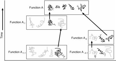
Figure 1. Evolutionist concept of gene origin by co-evolution. Boxes represent combinations of genes necessary for a particular function. Modified genes supposedly evolve a new function. Their previous function requires the origin of additional genes to be explained. (Black: protein residues present today; Dark grey: protein modifications, Light grey: hypothetical proteins needed by preceding functions.)
This poses a dilemma, since multiple other genes for the preceding function become necessary to explain the existence of a single subsequent gene. We thus replace one problem with a more difficult one (Figure 1).3 However, the materialist framework assumes biological complexity arises from simpler states.
Thousands of proteins appear to be dedicated to a single cellular function, in particular specialized enzymatic catalysis.4 There is no evidence they or related variants played another function earlier. One could hardly argue all genes or proteins in nature arose from a single master copy in a living organism. Examining sequences of proteins, which can range in length from a few dozen to 30,000 amino acids5 makes clear there are many families of sequentially unrelated proteins.
Let us neglect here the question of abiogenesis and assume some simple life form existed able to replicate successfully enough to not self-destruct. A theistic evolutionist might propose God used an evolutionary scheme without active guidance. Can natural genetic processes create novel, unrelated proteins over deep time?
Generating a novel protein family
Let us consider only a portion of this challenge: might a novel gene arise, able to code for a protein with just enough biological function (of any kind) to permit Darwinian selection to then begin fine-tuning the sequence. This is illustrated in Figure 2 (see ‘Cuttoff’ point). Evolution cannot look into the future and select for an organism having a random gene sequence which resembles ever so little that of a useful one to be developed, as has been assumed.1
All evolutionary computer models we are aware of neglect the low probability of random DNA sequences providing sequence instructions for a minimally useful, folded protein.1, 2, 6 Postulating preceding genes explains nothing. New families of unrelated genes must come from somewhere. It would be silly to argue nature kept duplicating a single original gene to produce the vast number of unrelated ones observed today. It does not help to argue sub-gene portions were already available, permitting ‘domain shuffling’, for the problem we are examining. In the evolutionary framework one would hardly argue the 31,474 known protein domains,7 as of 1 March 2001, were all available on the genomes of the earliest organisms. Furthermore, picking and choosing one or more members from this ensemble and attaching them to the correct portion of a gene is a hopelessly improbable endeavour.8
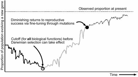
Figure 2. Hypothetical change in gene frequency of a population evolving a new gene from a duplicated gene.
Our hypothetical ancestor could resemble a bacterium. However, notice that these are usually not characterized as having large amounts of superfluous DNA for evolutionary experiments.
A minimally functional polypeptide
The protein with the greatest amount of sequence data available across organisms is cytochrome c. By lining the sequences up one notices that some residues are missing at some positions. Assuming these are dispensible we are left with a common denominator of 110 residues reported thus far in all organisms.9 An average protein is much larger than cytochrome c, consisting of about 350 amino acids.10 Let us examine whether a novel, minimally functional gene could develop de novo. One needs some genetic material to tinker with which is not bound to any critical biological function. We leave its source open to speculation but are not interested in producing a trivially similar gene from a copy of an already existing one. We would then simply enquire about the origin of the preceding gene.
Let us consider this new DNA portion a random base pair sequence. A process of trial-and-error is necessary to produce a minimally acceptable gene sequence before one can accelerate the convergence to a new gene using Darwinian selection arguments.11 Immediate biological value determines reproductive selectivity and not whether the sequence resembles a distant goal.1, 2,7
Chances of finding the first cytochrome c
In Appendix 1 we summarize Yockey’s probability calculations based on cytochrome c. Since some amino acids are used infrequently in nature, the realistic search space to generate functional proteins is smaller than that of all possible polypeptides of a given range of length. The reasoning is, chance would hardly ever produce polypeptides consisting of mostly those residues of low probability.
Since evolutionists assume this gene family is over 1 billion years old,12 there have been countless opportunities to generate all kinds of non-lethal variants. Yockey expanded the list of known sequences generously, using a model13 developed by Borstnik and Hofacker,14, 15 assuming many other sequences would also be tolerated even though not found in nature. The number of presumably acceptable cytochrome c protein sequences is given as (20) in Appendix 1.
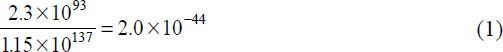
The ratio of minimally functional polypeptides to the subset of all sequences 110 amino acids long (excluding those of very low probability)16 provides us with an estimate of the proportion of minimally functional cytochrome c proteins before selective arguments can be invoked:
Alternative calculations to check plausibility
There are two alternative ways to estimate this proportion, both easier to understand. We determine the probability of obtaining an acceptable codon to code for a tolerated amino acid at each position of the protein, then multiply these probabilities together. Recall that the genetic code allows 1 to 6 codons to represent each amino acid. From the second column at the bottom of Table 2, Appendix 2 we found:

Alternatively, ignoring the proportion of synonymous codons used by the universal genetic code for each amino acid, and considering only the number of acceptable different amino acids out of 20 candidates leads to an estimate (Appendix 2, Table 2, last column at bottom of the table) of

This later approximation is reasonable for an abiogenesis scenario whereby amino acids are treated as being joined randomly (without a genetic code) and pretending only L-form amino acids exist.
Trials available to chance
The most favourable evolutionary scenario would involve organisms which reproduce asexually, such as by a budding or fission mechanism. To ensure cytochrome c gets transferred to the whole biosphere, our evolutionary scenario presupposes a single kind of bacteria-like creature. This has to take us back to well over a billion years before the Cambrian Explosion (which evolutionists place at around 550 million years ago) to ensure all life forms can have cytochrome c. In Appendix 3 we propose that an upper limit of 2x1042 attempts (25) could be made to produce a new gene in a billion years, although we had to use an unrealistically large, homogenous population; implausibly short average generation time; and a very rapid mutational rate which somehow avoids runaway self-destruction.
The number of available attempts (25) and proportion of sequences 110 amino acids long providing minimally functional cytochrome c (1) allows us to calculate the probability of stumbling on a useful variant of cytochrome c:

Discussion
An absurdly large population of rapidly reproducing organisms with high mutational rates for a billion years was assumed in (4) to favour the evolutionary model. Until minimal biological use has been attained for the evolving cytochrome c one cannot assume any kind of reproductive advantage arriving at this point. The analysis thus far casts serious doubt that the minimum requirements would be met for just one member of a novel biochemical process before Darwinian arguments even become relevant.
We shall defer to a later article the subsequent details of population genetics and fine-tuning of gene sequences.
From (4) it seems that even one very small protein is unlikely to arise by chance under the optimal conditions described. Should this occur against statistical odds, evolutionary processes must now begin the fine-tuning steps following the kick-in point in Figure 2. The fortunate organism now competes, with a small advantage against a large population calculated from (22) x (23) in Appendix 3 of:

members. Fisher’s analysis for sexually reproducing organisms showed that a favorable mutation with an unrealistically high selection coefficient of s = 0.1 would have only a 2% chance of fixing in a population of 10,000 or more.17
Since we only demanded that random mutations find a minimally functional cytochrome c to permit Darwinian selection to begin, an assumed s = 0.01 would be more than generous. Note that at least one mutant offspring must survive every generation or all is lost. We can envision a fission or budding reproductive model: on average, every 10 minutes the original bacterium either duplicates or dies (because the population is maximized in its environment). The probability the non-mutant will duplicate is p0 = 0.5. For the mutant, p0(1 + 0.01) = 0.505.
Assume the huge population postulated would allow a slight, localized increase in members, at least temporarily. The probability of the mutant surviving 1 generation is p = 0.505.
Having passed this hurdle, the n = 2 new mutants now have a probability of both dying given by the binomial probability distribution, using x= 0:
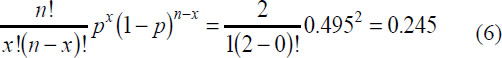
Thus, the novel mutation has a probability of only

of surviving just 2 generations. The chances are not good of fixing into the huge population.
Another consideration is that the build-up of mutants is initially very slow and stochastic, as shown in Figure 2. Since successful fission generates 2 members, the expected number of mutants after t generations is calculated as:

where p0 = 0.5.
Using s = 0.01 indicates that after 100 generations we expect on average to find only 2.7 mutants; using s = 0.001, a more realistic value, implies we’d need 1000 generations before 2.7 mutants would be found, on average.
However, survival chances can deviate greatly from the average over time, especially locally, due to several external factors. Within any litre of water, over millions of years the number of bacteria would shift by several percent countless times. Having assumed in (23) that there are 1x10¹¹ non-mutants initially per litre, it is unlikely all these would be exterminated world-wide.
But while the number of mutants is still small, such as 1 or 2 members, local difficulties for a few generations could easily wipe them all out even though we expect on average a positive s to lead to build-up. This only needs to happen once during the mutant build up time to destroy all evolutionary progress. This resembles investing in a single stock. The stock market over many years shows a buildup in value of around 10% per annum. Invest $1 initially and watch what the single stock does every 10 minutes. The evolutionary analogy is, if it falls under $1 just once, you must wait for a new generation to start all over again. The expected 10% growth over countless stocks and many years misrepresents the picture if during no 10 minute time slot are we allowed to fall under the original investment value ($1 or 1 survivor).
All evolutionary computer models we are aware of simplistically guarantee survival of those mutants which are supposed to evolve complex biological novelty1,2,6 and neglect the need to begin from ground zero again and again.
Note that the probability of obtaining additional useful mutations at precisely the site of the new gene is far lower than that of destructive ones accumulating anywhere on the genome. The odds of degrading any of the many finetuned genes which already exist is much greater than producing a fully functional new one.
Figure 2 illustrates another very important difficulty which we’ve never seen discussed in evolutionary models: the downward slope in proportion of ‘simple’ organisms, with fast generation times, possessing available DNA for evolutionary processes to experiment on. It is known18, 19, 20, 21, 22 that not having or losing superfluous genomic material offers measurable reproductive advantages. Less material and energy are required to duplicate the DNA, the potential for error is smaller and reproductive cycles are faster. This is particularly important if thereby worthless polypeptides no longer get produced: this saves energy and nutrients and avoids interference with necessary biological functions. 20–30% of a cell’s cytosol is composed of proteins and polypeptides not properly folded that can bond via hydrophobic interacions and gum up the cell.23 Prions are another example of the danger of having flawed polypeptides in the cell.
Fred Hoyle has worked out the mathematics of budding or binary fission reproduction in detail:24
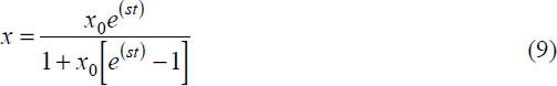
where x is the fraction of a population attempting to evolve a new gene; s is a selectivity factor; and the unit of time, t, is the generation interval.
To illustrate, suppose that at the beginning or during the billion years nature is trying to find a minimally function cytochrome c, 99.99% of the organisms possess “unnecessary” DNA material evolution can experimenting with: then x0 = 0.0001. Such “simple” genomes would now be on the order of 0.01% to 1% smaller. The advantages of not carrying extra ballast can be modelled as a faster rate of reproduction. Perhaps instead of 10 minutes their generation times are shortened by 0.1 second on average. We cannot do the experiments to determine what selectivity value, s, would result under natural conditions. Let us assume a very modest advantage of only s = 0.000167 (based on 0.1 / 600 seconds shortened generation time).
Now, we proposed a very short generation time to optimize the number of random attempts available to find a minimally functional novel gene by random mutations. But enough unnecessary DNA to permit cytochrome c to evolve now becomes a sizeable proportion of the genome, with severe penalties. In fact, from (9) on average the 0.01% would steadily reproduce more quickly and within 3 years become over 99.99999% of the whole population!25 Evolution is left with no superfluous DNA to experiment with. Admitedly, natural selection is not perfect, and local survivors could hold out longer. Novel genetic accidents might re-introduce unneeded DNA now and then. These would have to be of suitable size and not interfere with functional genes. Thereafter natural selection would again steadily favour the offspring able to discard chuncks of the new garbage, piece by piece.
Our assumed 0.1 seconds shortened generation time can be justified using merely one experimentally known fact. Each of 2 growing forks on E. coli can replicate less than 1000 base pairs (bps) of DNA per second.26 Since a new, cytochrome c size gene, complete with control regions, would require about 400 bps, having two forks now requires an additional 0.2 seconds to duplicate the genome. Ceteris paribus, the mutant lineages of rapidly reproducing organisms, carrying extra DNA to evolve a novel gene, would duplicate less efficiently.
Natural selection would remove DNA which is not immediately needed from rapidly reproducing populations with very small genomes. Thus suitable genetic material, in terms of size and location, to attempt to evolve cytochrome c, would disappear long before the billion years of evolutionary trials our scenario assumed.
Are the assumptions realistic?
The assumptions used were generous to allow a clear decision to be made. It is easy to demonstrate that a novel gene is more likely to arise and be fixed in huge populations than very small ones: the smaller number of trials available per generation time are not compensated for by subsequent more rapid fixing in smaller populations.
The evolutionist treats mutations as approximately random to avoid the risk of teleology. Furthermore, any factors facilitating de novo generation of our favourite gene would decrease the probability of creating those with unrelated sequences. The only potential for doubt lies in whether the proportion of minimally functional cytochrome c to worthless polypeptides, 2.0x10-44 from (1), is understated.
Alternatively, the 2.0x10-44, which is based on protein sequences, might actually be too generous when we consider its coding gene, which is what is relevant for evolutionary purposes, for several reasons:
-
Proteins must be generated in an acceptable proportion in the cell: a single copy has no value, and runaway production would be deadly. Regulation of gene transcription involves activators and repressors which bind at specific DNA sequences (combinations of the bases A,C,G, and T) near the gene. Each identifying sequence typically ranges between 5 to 40 bases. Sometimes a sequence must be precisely correct, other times 2 or more alternative bases are allowed at some positions. Binding of too many or incorrect regulatory proteins due to misidentification of binding sites must be prevented. Countless evolutionary trial and error attempts must thus also ensure too many addresses aren’t generated elsewhere on the genome: at best this would demand excess regulatory proteins, at worse it would prevent correct gene expression. In addition to suitable regulatory sequences to control and identify where a gene starts and ends, there are constraints with respect to the positioning of the binding sites with respect to the gene’s coding region.
Let us assume that only 2 binding sites, each 5 bases long and invariant, must be present to allow proper docking of 2 proteins which regulate expression of our new evolving gene.27 We neglect the spatial requirements with respect to the gene being regulated; where the regulatory proteins came from, and the need to eliminate false binding addresses from the genome. Merely requiring these 2 binding addresses decreases the probability of obtaining a minimally functional gene by a factor of:

This must also be taken into account if new genes are to be generated by first duplicating another one. Not only must new useful functions be created by mutating the preceding sequence, but independence from the regulatory scheme of the original copy demands novel binding sites for regulatory proteins. These must be produced by random mutations and simultaneously coordinated with the accompanying 3-dimensional structure of the co-evolving regulatory proteins, to permit physical interaction required by our new gene.
-
Known cytochrome c proteins were taken from a wide range of organisms for all known functions of the protein. Whether all organisms could make use of all these varieties is questionable, as also pointed out by Yockey.28, 29
-
iii) Yockey assumed all residues theoretically tolerable would be mutually compatible. A final 3-dimensional protein structure might indeed be consistent with alternative amino acids. But it is not certain all these possibilites would permit acceptable folding order46 to generate the intended protein structure.
-
iv) Although none of the three ‘Stop’ or ‘Terminator’ codons are expressed in the protein, one must be placed correctly on the gene. DNA sequences producing polypeptides not almost exactly 110 amino acids long won’t generate minimally functional cytochrome c.
This also decreases the proportion of acceptable candidates.
Plausibility of the evolutionary framework
We have now established considerable doubt as to whether natural processes or chance alone would generate a new gene family of even very small protein size. There are genes which show far less variability than cytochrome c, such as histones and ubiquitin, and most genes are much larger than cytochrome c. One could also analyze only a portion of a protein,30 such as the 260-residue highly conserved core of protein kinases. These examples have probability proportions vastly smaller than the 2.0 x 10-44 calculated in (1) and minimally functional members clearly could not have arisen by trial and error attempts.
When one looks at cellular processes which require multiple, unrelated proteins, one needs to realize that the chances of obtaining these by chance are the individual probabilities multiplied together. For example, bacterial operons are clusters of contiguous genes transcribed as a unit, from which multiple proteins are generated. From the tryptophan operon five proteins are generated for a single cellular process: manufacture of tryptophan when needed. This scheme ensures the proteins get generated in the same relative proportion.31 The odds of producing operons consisting of n genes by chance is roughly that of creating the average gene sequence raised to the nth power.32 We are not aware of any claims of any operon having biological functionality with less than all n gene members simultaneously. Operons appear to be ‘irreducibly complex’ and cannot arise stepwise.
The proportion of functional protein sequences is sometimes very small due to complex interactions with other proteins.33 Alternatively, this is perhaps easier to understand for the thousands of proteins used as dedicated enzymes: a specialized three-dimensional cavity must be generated whose spatial and electronic structure fits the transition state of a specific chemical reaction, like a hand and glove. This lowers the energy requirement to produce the rate determining intermediate and can accelerate the overall reaction by a factor of millions. The portion of the protein not directly involved in the catalysis is needed to ensure that a stable structure gets generated reproducibly, and other portions may be needed to ensure a correct folding order over time to produce the mature protein. Other domains may be required to ensure correct interaction with other proteins or to direct the biomolecule to specific portions of the cell.
Minimum number of genes needed
Parasitic mycoplasms, although not free-living cells, are used in studies to estimate the minimal number of genes needed for a living organism, at least under careful life support laboratory conditions. Genes are knocked out deliberately to see which one’s number are temporarily dispensible. Estimates for the lowest range between 250– 400 genes.34 Obtaining multiple, unrelated genes by chance (which together provide the minimum functionality to survive) has an overall probability approximately equal to multiplying the individual probabilities of forming each gene together. If these had the length and variability characteristics proposed for cytochrome c, the minimal requirements to barely survive (already in a suitable membrane, with energy and nutritional needs provided, with translation and transcription somehow already functional) is of the order of 1x10(-44)(300) which one can safely state did not occur by trial and error (assuming a minimal cell of 300 proteins).
Troublesome prediction for an evolutionist
Evolutionary theory demands that if thousands of distinct gene families were not present concurrently in the original common ancestor then these had to have been generated over time. Evidence of evolutionary tinkering in the process of producing new gene functions should be everywhere.
As pointed out above, one cannot argue that every cellular and biological function is connected to some preceding one. This would theoretically permit an evolving gene to support one function even as another is being prepared. Then in the twinkling of an eye the gene discontinues function A-2 and concentrates on A-1. However, many cellular processes show no resemblance to any other known. No bridges among them are known nor conceivable. Evolutionary theory makes clear that a molecular biologist who discovers a new gene has no justification to expect it to demonstrate a current biological use. The evolutionary history of genes would be characterized by predominantly pre-functional stages. Note how scientifically stiffling consistent application of evolutionary belief becomes. There would be little motivation to keep seeking the purpose of novel genes since most would probably not yet have one. Nevertheless, it is interesting to note that biologists inevitably assume a newly discovered gene will be shown to have some current purpose.
Various scientific questions need to be addressed within the creationist paradigm. (Figure 3). How much variability within gene families was present within a genome and across Biblical kinds immediately post-Flood is not known. We suspect much variability was already present across organisms, reflecting different needs and environments. The Fall predicts introduction of flaws. Severe bottlenecks (which eliminated many members with better genes) and deleterious environmental factors during and after the Flood would have facilitated the spread of many damaging mutations. We suggest that empty ecological niches and rapidly growing populations allowed a larger proportion of flawed genomes to be tolerated. Geographic isolation permitted genetic pool fragmentation. Natural selection could only weed out dramatic genetic failures and would operate in a wider range of contexts in the immediate post- Flood world. The overall effect would be far greater variability in gene sequences of less than optimal performance in a shorter time frame than expected from a uniformitarian world view.
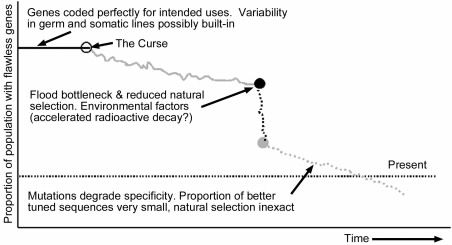
Figure 3. Creationist model: gene specificity for biological uses is degrading on average.
Natural selection cannot ensure pristine genomes by weeding out every flaw. The proportion of less specific sequences always greatly out-number the better. Survival is a very stochastic effect, and in our view the net effect of mutations is to destroy both specificity and function. This view predicts we may indeed find genes which no longer perform a useful function. Usually these would no longer generate m-RNA. Contra evolution, observation over many generations under natural conditions would show sequence randomization and not net improvement. Even under ideal laboratory conditions and accelerated, induced mutations, countless genetic experiments on fruit flies and rapidly duplicating E. coli have yet to produce a useful, informationincreasing mutation. Degrading mutations are rampant.
Conclusions
The proportion of gene sequences comparable to cytochrome c, having minimal biological functionality, has been estimated at 1 out of 5x1043 (from the reciprocal of (1)) sequences of appropriate DNA length. Since this would demand many mutational trials and errors, we favoured the evolutionary model by assuming a single bacteria-like organism with very short generation time; a huge population; asexual reproduction; plentiful nutrients; and a very high mutation rate (we neglected the effect on the rest of the genome). Theoretical pre-Cambrian organisms such as ancestor tribolites or clams, with much larger genomes, would (a) have generation times many orders of magnitude longer than our assumed 10 minutes, and (b) population sizes many orders of magnitude smaller. These facts together permit far fewer trial and error attempts. So if the case cannot be made for bacteria-like creatures then novel gene families did not arise by such evolutionary mechanisms.
We are not interested here in the origin of cytochrome c per se but in trying to determine what an evolutionary starting polypeptide for unrelated classes of genes35 might look like. One generally assumes a functional protein will consist of over 100 amino acids,36, 37 which is close in size to the protein we have examined. Rarely does one expect that on average over half of the 20 amino acids could be used at any amino acid site, as was done here. Might even cytochrome c have begun from a simpler ancestor gene? For the evolutionist this would only be interesting if it had even fewer constraints, which soon starts to border on the absurd. If too much flexibility is permitted for multiple functions then natural selection has no consistent criteria to work with.
Furthermore, it is questionable whether anything would be gained by presuming a yet simpler ancestor gene: the number of trials and errors to produce such the minimally useful protein would be indeed smaller. But now a very great number of generations are needed to mutate this useful gene, along with others, into a brand new biological function, as used by the present version. Instead of invoking an endless regress, let us accept that there needs to be a starting point for minimally useful genes.
Cellular research has revealed a level of complexity and sophistication not suspected by Darwin and subsequent evolutionary theorists. One reads of molecular machines38 to perform specific biological functions, composed of multiple independent parts working together in a highly coordinated manner.
The complete atomic structure of the large ribosomal subunit of Haloarcula marismortui was reported recently.39 It consists of over 3,000 nucleotides and 27 specialized proteins. It is an integral part of the ribosome machinery, present in multiple copies in every cell. This equipment decodes each messenger RNA many times to determine the order amino acids are to be linked together to generate proteins. Additional components are needed, such as a reliable energy source delivered at a suitable level to the correct place and the right time,40 to rachet41 through the mRNA one codon at a time.
Professor Behe identifies many examples of biological functions42, 43 which are ‘irreducibly complex’ since no biological use is possible until all components are present and finely meshed.
However, the proportion of minimally functional genes to worthless sequences of comparable length is very small. A proportion of »2x10-44 has been proposed for cytochrome c, an atypically small protein, but for which the largest set of protein sequences are available. Cassette mutagenesis studies44, 45 by Sauer allowed an estimate of the proportion of polypeptides able to fold properly,46 one requirement for proteins to be functional. For the cases studied, a proportion of about 10-65 was estimated, although no biological function was shown to exist even for that subset. This corresponds statistically to guessing correctly one atom in our galaxy.
In addition, gene expression requires specific sequences of bases in their vicinity to which preexisting regulatory proteins must bind. Trial and error mutations must both generate these addresses and eliminate incorrect ones from the genome.
Even with unrealistic assumptions it is unreasonable to claim mutations in the germ-lines (by design or chance) produced the large number of protein families found. We base this conclusion on merely the unlikelihood of one single, novel gene arising upon which evolutionary mechanisms could begin to work. Our calculations are not to create well-tuned gene sequences optimally expressed, but merely the hurdles to be overcome before Darwinian fine-tuning arguments even have any relevance.
The integration of multiple, unrelated proteins to produce thousands of distinct cellular functions is best explained by a deliberate and planned creative act.
Acknowledgements
Extensive correspondence with Hubert Yockey clarified several difficulties. We look forward to the second edition of his book. We thank the anonymous reviewers cooperating with Answers in Genesis for critical comments and analysis.
Appendix 1
The size of the polypeptide search space The number of possible sequences using n amino acids is given by 20 x 20 x 20 . . . n times. For the subset of n = 110 residues of cytochrome c this indicates

candidate amino acid sequences.
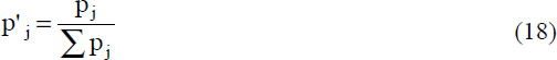
Now, the proportion of each amino acid used by proteins varies significantly. Yockey47 showed that to a good approximation the number of synonymous codons allows a good estimate for the frequency each amino acid is used by proteins, except for arginine (Table 1). Then the probability, pj, of finding an amino acid at a specific position, j, is affected by an existing genetic code and to a first approximation,

where rjrepresents the number of codons (between 1 and 6) coding for amino acid j and pi= 1/61, the codon probability, as explained in Table 1.
| Reside | Probability, Pi | Calculated Value | King & Jukes | Goel et al. |
|---|---|---|---|---|
| leu | p1 | 6/61 = 0.0984 | 0.076 | 0.0809 |
| ser | p2 | 6/61 = 0.0984 | 0.081 | 0.0750 |
| arg | p3 | 6/61 = 0.0984(b} | 0.042 | 0.0419 |
| ala | p4 | 4/61 = 0.0656 | 0.074 | 0.0845 |
| val | p5 | 4/61 = 0.0656 | 0.068 | 0.0688 |
| pro | p6 | 4/61 = 0.0656 | 0.068 | 0.0494 |
| thr | p7 | 4/61 = 0.0656 | 0.062 | 0.0634 |
| gly | p8 | 4/61 = 0.0656 | 0.074 | 0.0748 |
| ileu | p9 | 3/61 = 0.0492 | 0.038 | 0.0458 |
| term | p10 | 0 = 0(c) | 0 | 0 |
| tyr | p11 | 2/61 = 0.0328 | 0.033 | 0.0345 |
| his | p12 | 2/61 = 0.0328 | 0.029 | 0.0222 |
| gln | p13 | 2/61 = 0.0328 | 0.037 | 0.0413 |
| asn | p14 | 2/61 = 0.0328 | 0.044 | 0.0535 |
| lys | p15 | 2/61 = 0.0328 | 0.072 | 0.0605 |
| asp | p16 | 2/61 = 0.0328 | 0.059 | 0.0555 |
| glu | p17 | 2/61 = 0.0328 | 0.058 | 0.0538 |
| cys | p18 | 2/61 = 0.0328 | 0.033 | 0.0230 |
| phe | p19 | 2/61 = 0.0328 | 0.040 | 0.0402 |
| trp | p20 | 1/61 = 0.0164 | 0.013 | 0.0153 |
| Met | p21 | 1/61 = 0.0164 | 0.018 | 0.0155 |
Polypeptides composed mostly of amino acids of low occurrence are very unlikely to exist. The odds of obtaining a polypeptide n=110 residues long based on only residues represented by 1 codon (such as trp and met, with chances of ca. 1/61) compared to one based on only residues represented by 6 codons (such as leu and ser, with odds of 6/61), is:
For n greater than 110 residues this proportion drops rapidly.48
Treating the genetic code as given, it appears that the search space given by (11), in the absence of intelligent guidance, is exaggerated since many worthless, but highly improbable, candidates would not be tested by chance. One can define two collections of sequences, one consisting of those polypeptides which as a collection possess negligible chance of being generated compared to the second, higher probability set.
We avail ourselves of some mathematics developed by Shannon for telecommunication purposes and applied by Yockey to the analysis of gene and protein sequences.49
The entropy, H, for each residue position of a protein can be calculated by:

which gives H = 4.139 ‘bits’ using pj from (12).
The number of different polypeptides using n amino acids, neglecting the set of those belonging to the very low probability class, is given by

where a = 2, if we choose to work with base 2 logarithms, which is mathematically convenient. This reduces the potential search space suggested by (11) to

candidate polypeptides of length 110 amino acids. Were the probability of obtaining any amino acid identical, meaning 1/20 for every position, then equations (14) and (15) would predict the same number of candidate sequences, (20) 110, as found in (11).
The set of functional cytochrome c sequences.
We restrict ourselves now to single protein family, cytochrome c. The entropy, H, of the probability distribution of the synonymous residues at any site l is given by

where
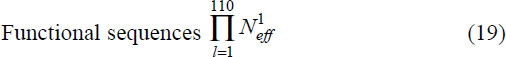
The summation in (18) includes only the synonymous residues, based on available sequence data, at position l on the polypeptide. pj was defined in (12). The effective number of synonymous residues at each site l is calculated as:

where H1 is defined in (17). Finally, multiplying these values for all 110 sites provides the number of known functional cytochrome c variants:
It is possible additional sequences will be discovered, may have gone extinct, or would be functional but have not been produced by mutations. This potential was estimated using a prescription developed by Borstnik and Hofacker.14 20 amino acid physical properties were used, from which 3 orthogonal eigenvectors were sufficient to describe the data adequately. This differs from an earlier approach47, 49, 50 which was based on Grantham’s51 prescription.
The estimated functional sequences reported52 are

Appendix 2
Alternative calculations of probability to obtain a funtional cytochrome c protein
The amino acids presumed to be tolerated at each position on the protein is used, along with the probability of generating the acceptable amino acid (based on synonymous codons from the universal genetic code). Then it is straightforward to calculate the odds of finding an acceptable residue for each position. This is provided in the column labelled Spi at the bottom of Table 2. Multiplying the individual probabilities leads to an overall probability of

of obtaining a minimally functional cytochrome c protein.
This simplification could be justified by that fact that generally the proportion of a particular amino acid in proteins does parallel fairly well the number of codons assigned to it, see Table 1. Yockey’s more rigorous mathematics, which removes from consideration polypeptide sequences of very low probability, leads to an estimated of 2.0 x 10-44, see (1).
A simpler alternative ignores the number of synonymous codons used by the universal genetic code and considers only the number of acceptable amino acids at each protein site. This leads to an estimate (last column, bottom of Table 2) of

As a back-of-the-envelop estimate this later approach is useful as a rough orientation. It has relevance for abiogenesis scenarios when: only the 20 amino acids are present; in relative proportions reflecting usage in proteins; in the absence of interfering reactants, including water; only L form amino acids are present; no chemical side-reactions occurs (such as intramolecular rings, condensation of side chain carboxylic acids, oxidation reactions, etc.).
Appendix 3
Trials available to chance
How many opportunities might chance have to stumble on a functional cytochrome c sequence? We permit all random mutational processes able to generate a new sequence on a suitable portion of DNA not needed for other purposes. Let us assume some generous settings from an evolutionary perspective to avoid argument:

based on 1 generation per 10 minutes on average for 1 billion years. For comparison, ‘In ideal growth conditions, the bacterial cell cycle is repeated every 30 minutes’.53 Our proposed value is surely about a factor of 10 too generous on average.

based on an assumed primitive ocean of volume 20,000 x 20,000 x 1 km. The current oceans are believed to contain about 1.4 x 10²⁰ litres of water:54
Since the ancient earth framework assumes water accumulated from comets and water vapour from volcano eruptions over billions of years, the putative aqueous living space would actually have been on the order of only 1/10th the volume we are using.
| Site Nr(b) |
pj:(a) | Ala 4/ 61 |
Arg 6/ 61 |
Asn 2/ 61 |
Asp 2/ 61 |
Cys 2/ 61 |
Gln 2/ 16 |
Glu 2/ 16 |
Gly 4/ 61 |
His 2/ 61 |
Ile 3/ 61 |
Leu 6/ 61 |
Lys 2/ 61 |
Met 1/ 61 |
Phe 2/ 61 |
Pro 4/ 61 |
Ser 6/ 61 |
Tyr 2/ 61 |
Trp 4/ 61 |
Thr 4/ 61 |
Val 4/ 61 |
|---|---|---|---|---|---|---|---|---|---|---|---|---|---|---|---|---|---|---|---|---|---|
| 23 | 1 | 1 | 1 | 1 | 1 | 1 | 1 | 1 | 1 | 1 | 1 | 1 | 1 | 1 | 1 | ||||||
| 36 | 1 | 1 | 1 | 1 | 1 | 1 | 1 | 1 | 1 | 1 | 1 | 1 | 1 | 1 | 1 | ||||||
| . . . | |||||||||||||||||||||
| 34 | 1 | 1 | 1 | 1 | 1 | 1 | 1 | 1 | |||||||||||||
| 38 | 1 | ||||||||||||||||||||
| 40 | 1 | ||||||||||||||||||||
| . . . | |||||||||||||||||||||
| 17 | 1 | 1 | 1 | 1 | 1 | 1 | 1 | 1 | 1 | 1 | 1 | 1 | 1 | 1 | 1 | 1 | 1 | ||||
| 35 | 1 | 1 | 1 | 1 | 1 | 1 | 1 | 1 | 1 | 1 | 1 |
| Site Nr(b) |
Σpj(c) | H1(d) | 2H1=N1eff | AAs(e) | Prob.(f) |
|---|---|---|---|---|---|
| 23 | 0.787 | 3.7563 | 13.513 | 15 | 0.75 |
| 36 | 0.787 | 3.7563 | 13.513 | 15 | 0.75 |
| . . . | |||||
| 34 | 0.328 | 2.8464 | 7.192 | 8 | 0.4 |
| 38 | 0.066 | 0 | 1 | 1 | 0.05 |
| 40 | 0.098 | 0 | 1 | 1 | 0.05 |
| . . . | |||||
| 17 | 0.885 | 3.9163 | 15.098 | 17 | 0.85 |
| 35 | 0.541 | 3.2559 | 9.553 | 11 | 0.55 |
| Prob.: | 2.71x10-44 | 310.1508 bits | Probl.: | 6.88x10-45 |
One evolutionist would like to enlighten us55 that such a primitive ocean would have contained 1 x 1024 litres of water, conveniently stocked full of just the right 20 amino acids. Which is more probable, his claim or (22)? Post French Revolution the circumference of the earth was measured at 40,000 km. 1 thousandth of a km became the definition of a metre and a cube of 1/10th of a metre full of water became the definition of a kilogramm. A litre is a cube having length 1/10th of a metre.
If the earth were a perfect sphere the measured circumference would indicate a radius of about 6,366.2 km. Using the accepted radius54 of 6,378.15 km and assuming a perfect sphere provides an estimate of the earth’s total volume:

For the evolutionist’s statement55 to be true the whole earth would have to consist of water, clearly absurd.
As an alternative calculation to see whether (22) is reasonable let us assume there were no continents and the ocean had an average of 1 km depth. The outer radius r1 is 6378.15 km and the inner radius r2 is (6378.15 - 1) km This would provided a volume of water:

This confirms that (22) has been deliberately exaggeraged to favour the evolutionary scenario.

based on 10% of the levels available for concentrated E. coli under optimal laboratory conditions.56 We assume sufficient nutrients are available in nature during the billion years and that this high concentration was maintained from water surface to a depth of 1 km. On average over a billion years this is probably at least 100 times too generous.
Note that the maximum number of organisms thus estimated agrees almost precisely with other work performed independently.57

Estimates of error rates during DNA duplication vary. Yockey58 suggested between 10-7 and 10-12 per nucleotide. Other literature indicate between 10-7 and 10-10.59, 60, 61, 62 Using the fastest mutation rate proposed in the literature above indicates about 3.3 x 10⁻⁵ base pair changes per generation, based on:

Let us by generous and use a mutation rate of 1 per 1000 generations, which is about 30 times greater than the fastest estimate proposed to avoid argument. Furthermore we will neglect the effect such random mutations would have on the rest of the genome.
These assumptions offer a generous maximum number of attempts possible:

mutational opportunities.
has bachelor’s degrees in chemistry and in computer science from State University of New York; an MBA from the University of Michigan; and a Ph.D. in organic chemistry from Michigan State University. He works for BASF in Germany.
completed his State Exam (which corresponds to a Masters of Science) in food science from the University of Karlsruhe and doctorate in molecular biology from the University of Freiburg. He currently works at the University of Heidelberg, Germany.
Footnotes
- Dawkins, R., The Blind Watchmaker, Penguin Books, London, 1986; Dawkins, R., New Scientist, 34, 25 September 1986.
- Schneider, T. D., Nucleic Acids Res., 28:2794, 2000.
- Either all gene families existed in the earliest living organisms or new ones have arisen. Movable genetic elements, within the genome and across unrelated species, could be a designed process to introduce variety. Research may clarify this possibility. But it is not productive from an evolutionary perspective to argue all new biological functions arose from earlier states which require yet more genes. There are many processes which involve several genes not used for any other purpose. An evolving gene requiring cooperation with other genes already in use is faced with formidable cooperative challenges, especially since all improvements rely on random mutations. Any damaged on-going services would be selected against for that organism. Novel functions would have to develop almost instantly to prevent mutational destruction of new genes in the process of evolving.
- Lodish et al., Molecular Cell Biology, 4th ed., W. H. Freeman and Company, New York, p. 70, 2000: ‘an animal cell, for example, normally contains 1000–4000 different types of enzymes, each of which catalyzes a single chemical reaction or set of closely related reactions.’
- Lodish et al., Ref. 4, p. 125.
- Küppers, B-O., The prior probability of the e of life; in: Krüger, L., Gigenrenzer, G. and Mortgan, M.S. (Eds), The Probabilistic Revolution, MIT, Press, Cambridge, pp. 355–369, 1987. Discussed by S. Meyer in Ref. 42, p. 80–82.
- Structural Classification of Proteins (SCOP), <scop.mrc-lmb.cam.ac.uk/scop/>. Domains are portions of proteins with distinct geometric themes, typically 50–100,10 or according to Ref. 30, 100–200, residues large. These generic features can be found across different proteins and do not require identical residues. The chemical significance and biological use can often by deduced by examining such portions of proteins. We view this as the handiwork of the Master Engineer who used the same generic components for many purposes. It is not surprising that a domain known to attach to hydrophobic surfaces, like the interior of membranes, appears in proteins which must perform such functions.
- Portions of genes coding for a domain would have to be precisely extracted. Proteins can have one or more copies of each of n domains. Correctly choosing n = 2 specific domains by chance to build a new gene has a probability of 1 out of 9.9 x 10⁸ (i.e., (31,474)2 )) , assuming both domain-coding regions happened to be suitably extracted). Both must then be introduced into an acceptable portion on a chromosome which does not interfere with existing genes. Proteins with N = 5 domains and larger are not unusual. (31,474)5= 3.2 x 10²³ correct choices are now required, placed suitably with respect to each other. If such wild and random genetic scrambling were common the genome could not last very long.
- Yockey, H.P., Information Theory and Molecular Biology, Cambridge University Press, Cambridge, p. 250, 1992.
- Doolittle, R.F., Annu. Rev. Biochem., 64:287, 1995.
- It is not plausible to argue genes free themselves from one function, then assume a new one without transversing a non-functional stage. Complex biological functions are not connected by unbroken topologies. In Ref. 1, Professor Dawkins simply assumes that there is an unbroken chain of mutations leading from a random state to a complex organ such as an eye, each possessing a selective advantage.
- Yockey, Ref. 9, p. 135.
- Yockey, Ref. 9, p. 136.
- Borstnik, B. and Hofacker, G.L.; in: Clementi, E., Corongiu, G., Sarma M.H. and Sarma, R.H. (Eds), Structure & Motion, Nucleic Acids & Proteins, Guilderland, Adenine Press, New York 1985.
- Borstnik, B., Pumpernik, D. and Hofacker, G.L., Point mutations as an optimal search process in biological evolution, J. Theoretical Biology 125, 249–268, 1987.
- Yockey, Ref. 9, p. 254.
- Fisher, R.A., The Genetical Theory of Natural Selection, 2nd revised edition, Oxford University Press, Oxford, New York, Dover, 1958.
- Shapiro, R., Origins: A Skeptic’s Guide to the Creation of Life on Earth, Bantam Books, New York, pp.157–160, 1987. The Qb parasite genome uses a single strand of RNA with 4,500 nucleotides. Sol Spiegelman (University of Illinois) placed Qb, a necessary replicase and certain salts in a test tube. Portions of the genome dispensible in this environment were lost, permitting their offspring to reproduce more quickly. After about 70 generations everything superfluous had been eliminated, and a single species with a single RNA strand 550 nucleotides long remained. In a second experiment (p. 160), RNA already shortened optimally was allowed to replicate in the presence of a drug that slowed down replication. The drug attached to a specific three nucleotide sequences. After a few generations all members possessed the same, new sequence, in which the recognizer address for the drug had mutated to 3 other nucleotides, preventing drug binding and permitting faster reproduction.
- Lodish et al., Ref. 4, p. 187. ‘The fusion of two cells that are genetically different yields a hybrid cell called a heterokaryon.’ ‘As the humanmouse hybrid cells grow and divide, they gradually lose human chromosomes in random order, but retain the mouse chromosomes. In a medium that can support growth of both the human cells and mutant mouse cells, the hybrids eventually lose all human chromosomes. However, in a medium lacking the essential metabolite that the mouse cells cannot produce, the one human chromosome that contains the gene encoding the needed enzyme will be retained, because any hybrid cells that lose it following mitosis will die.’
- Beaton, M.J. and Cavalier-Smith, T., Proceedings of the Royal Society (B), 2656:2053, 1999. Cryptomonads can remove functionless DNA (pointed out in Ref. 22, p. 8).
- Petrov et al., Molecular Biology Evolution, 15:1592, 1998. Drosophilia can remove functionless DNA (pointed out in Ref. 22, p. 8).
- Darrall, N.M., Origins: The Journal of the Biblical Creation Society, 29:2, 2000.
- Lodish et al., Ref. 4, p. 63: ‘More than 95 percent of the proteins present within cells have been shown to be in their native conformation, despite high protein concentrations (»100 mg/ml), which usually cause proteins to precipitate in vitro.’
- Hoyle, F., Mathematics of Evolution, Acorn Enterprises LLC, Memphis, 1999. Use equation (1.6) on p. 11.
- For t in equation (9) use: (6 generations/hour) x (24 hours/day) x (1095 days/3 years) = 157680 generations in 3 years.
- Lodish et al., Ref. 4, p. 456.
- In addition to promotor sites, regulation of gene expression and modification of mRNA can require multiple base pair sequences which do not encode for proteins. Lodish et al., Ref. 4, p. 295: ‘Other critical noncoding regions in eukaryotic genes are the sequences that specify 3’ cleavage and polyadenylation [poly(A) sites] and splicing of primary RNA trnascriptions.’ p. 413: ‘Nearly all mRNA contain the sequence AAUAAA 10–35 nucleotides upstream from the poly(A) tail.’
- Pennisi, Ref. 42, p. 346: ‘Fitsch & Markowitz (1970) have shown that as the taxonomic group is restricted the number of invariant positions increases.’
- Yockey, Ref. 9 p. 315.
- Lodish et al., Ref. 4, p. 60: ‘A structural domain consists of 100–200 residues in various combinations of a helices, b sheets, and random coils.’
- Lodish et al., Ref. 4, p. 405. The tryptophan operon encodes the enzymes necessary for the stepwise synthesis of tryptophan. From the single operon an mRNA strand is produced which gets translated into the 5 proteins (E,D,C,B,A) needed. Proteins E and D form the first enzyme needed in the biosynthetic pathway; C catalyzes the intermediate; B and A combine to form the last enzyme needed. ‘Thus the order of the genes in the bacterial genome parallels the sequential function of the encoded proteins in the tryptophan pathway.’ Ref. 5, p.144.
- Actually, the odds are worse. For example: the odds of getting two events with probability 0.5 is: 0.5 x 0.5 = 0.25 whereas having probabilities of 0.25 and 0.75 is less: 0.25 x 0.75 = 0.19. Probabilities of 0.01 and 0.99 leads to 0.009 although the ‘average’ in all cases is 0.5. One could badly overestimate probabilities when told that a large protein has much freedom in most of its positions. A few invariant positions make a huge difference. Examination of Yockey’s data (Ref. 9, Table 9.1) reveals that on average 10.9 (out of 20 possible amino acids) are expected to be tolerated at each position. Therefore, an unusually restrictive, or ‘conserved’ protein has not been examined here. However, 16 of the 110 positions (14.5.%) require a specific amino acid. Neglecting the fact that the genetic code favours some amino acids, the odds of getting all 16 invariant positions is roughly (1/20)16 = 1.5x10⁻²¹. An average protein about 3 times larger than cytochorme c with 330 residues and a comparable 14.5% invariant sites could have (330-48) = 282 sites where any amino acid is allowed, clearly a very undemanding protein. Nevertheless, requiring 48 invariant sites by random mutations has roughly a chance of (1/20)48 = 3.7 x 10-63. This is vastly less likely than Yockey calculated for the entire cytochrome c protein.
- Kirschner, M. and Gerhart, J., Proc. Natl. Acad. Sci. USA, 96:8420, 1998.
- Pennisi, E., Science, 272:1098, 1996; Mushegian, A. and Koonin, E., Proc. Nat. Acad. Sci. USA, 93:10268, 1996; Bult, C. et al., Science, 273:1058, 1996. Discussed in Fisher, Ref. 18, p. 76. Creationist professor emeritus Dr Roland Süßmuth is a specialist in mycoplasms and presented a paper on this topic at the 18th Creationist Biology Conference, Süßmuth, R., Die Bakteriengruppe der Mycoplasma, Tagesband der 18. Fachtagung für Biologie, p. 69, 16– 18 März 2001. Studiengemeinschaft Wort und Wissen e.V. Rosenbergweg 29, D-72270, Baiersbronn, Germany.
- Lodish et al., Ref. 4, p. 299 (Discussing gene families) ‘Most families, however, include from just a few to 30 or so members; common examples are cytoskeletal proteins, 70-kDA heat-shock proteins, myosin heavy chains, chicken ovalbumin, and the a- and b-globins in vertebrates.’ Proteins from sequentially unrelated genes are often involved in jointly providing biological functions. For example, Ref. 5, p. 300: ‘Several different gene families encode the various proteins that make up the cytoskeleton.’
- Lodish et al., Ref. 4, p. 283: ‘This gene-knockout approach already has been used to analyze yeast chromosome III. Analysis of the DNA sequence indicated that this chromosome contains 182 open reading frames of sufficient length to encode proteins longer than 100 amino acids, which is assumed in this analysis to be the minimum length of a naturally occurring protein’ (emphasis added).
- Lodish et al., Ref. 4, p. 236: ‘An ORF [Open Reading Frame] is a DNA sequence that can be divided into triplet codons without any intervening stop codons. Although some polypeptides are shorter than 100 amino acids, these are difficult to predict from DNA sequences alone because short ORFs occur randomly in a long DNA sequence. Long ORFs encoding 100 or more amino acids are unlikely to occur randomly and very likely encode an expressed polypeptide.’
- Alberts, B., Cell, 92:291, 1998.
- Ban, N., Nissen, P., Hansen, J., Moore, P.B. and Steitz, T.A., Science, 289:905, 2000.
- Bergman, J., CRSQ, 36(1):2, 1999.
- Frank, J. and Agrawal, R.K., Nature, 406:318, 2000.
- Behe, M.J., Dembski, W.A. and Meyer, S.C., Science and Evidence for Design in the Universe, Ignatius, San Francisco, 2000. 43.
- Behe, M.J., Darwin’s Black Box: The Biochemical Challenge to Evolution, Touchstone, New York, 1996.
- Reidhaar-Olson, J. and Sauer, R., Proteins, Structure, Function and Genetics, 7:306, 1990; Bowie, J. and Sauer, R., Proc. Nat. Acad. Sci. USA 86:2152, 1989; Bowie, J., Reidhaar-Olson, J., Lim, W. and Sauer, R., Science, 247:1306, 1990; Behe, M., Experimental support for regarding functional classes of proteins to be highly isolated from each other; in: Buell J. and Hearns, G. (Eds), Darwinism: Science of Philosophy? Haughton Publishers, Dallas, pp. 60–71, 1994; discussed in Ref. 42, p. 75.
- Axe, D., Foster, N. and Ferst, A., Proc. Nat. Acad. Sci. USA 93:5590, 1996. Discussed in Ref. 42, p. 75.
- Lodish et al., Ref. 4, p. 62: ‘Any polypeptide chain containing n residues could, in principle, fold into 8n conformations.’
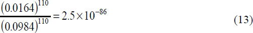
- Yockey, H.P., J. Theor. Biol. 46: 369, 1974; p. 381.
- One sees how quickly the proportion drops with increasing polypeptide length, n, by taking the log of the ratio: proportion = 10n[log0.0164 - log 0.0984] = 10-0.778n
- Yockey, H.P., J. Theor. Biol. 67:377, 1977.
- Yockey, H.P., J. Theor. Biol., 67:345, 1977; see p. 361.
- Grantham, R., Science, 185:862, 1974.
- Pennisi, Ref. 9, p.254.
- Lodish et al., Ref. 5, p. 9.
- ‘Earth’, <seds.lpl.arizona.edu/nineplanets/nineplanets/earth.html>.
- Musgrave, I., Lies, damned lies, statistics, and probability of abiogenesis calculations, <www.talkorigins.org/faqs/abioprob.html>.
- Personal communication from Professor Scott Minnich, email from 17 March 2001.
- Scherer, S. and Loewe, L., Evolution als Schöpfung? in: Weingartner, P. (Ed.), Ein Streitgespräch zwischen Philosophen, Theologen und Naturwissenschaftlern, Verlag W. Kohlhammer, Stuttgart; Berlin; Köln: Köhlhammer, pp. 160–186, 2001. The authors were made aware of the above essay just prior to the submission of this paper. It contains many valuable probability calculations performed independently and unknown to us. It is reassuring that although they worked with different assumptions, virtually identical numbers resulted. For example, they calculated the maximum number of cells which could have lived in 4 billion years as 1046 whereas we estimated for 1 billion years, 2 x 1045 : From Appendix 3: (5 x 10¹³)(4 x 10²⁰)(1 x 10¹¹) = 2 x 1045.
- Yockey, Ref. 9, p. 301.
- In bacteria the mutation rate per nucleotide has been estimated to be between 0.1 and 10 per billion transcriptions.60,61 For organisms other than bacteria, the mutation rate is between 0.01 and 1 per billion.62 References found in: Spetner, L., Not by Chance! Shattering the Modern Theory of Evolution, The Judaica Press, Inc., Chapter 4, 1998.
- Fersht, A.R., Proceedings of the Royal Society (London), B 212:351–379, 1981.
- Drake, J.W., Annual Reviews of Genetics, 25, 125–146, 1991.
- Grosse, F., Krauss, G., Knill-Jones, J.W. and Fersht, A.R., Advances in Experimental Medicine and Biology, 179:535–540, 1984.
- Yockey, Ref. 9, p. 250.
- Hampsey, D.M., Das, G. and Sherman, F., J. Biological Chemistry 261:3259, 1986.
- Hampsey, D.M., Das, G. and Sherman, F., FEBS Letters 231:275, 1988.
- Yockey, Ref. 9, p. 162.
- Yockey, Ref. 9, p. 250.
Support the creation/gospel message by donating or getting involved!

Answers in Genesis is an apologetics ministry, dedicated to helping Christians defend their faith and proclaim the good news of Jesus Christ.
- Customer Service 800.778.3390
- Available Monday–Friday | 9 AM–5 PM ET
- © 2026 Answers in Genesis