

Appendix
by
Dr. Danny R. Faulkner
on
July 16, 2013
Republished with permission and featured in
Universe by Design
Modern astronomy allows us to find the distances, sizes, temperatures, and masses of stars. This is incredible, given how far stars are from us.
Spectra of Light
Almost all that we know about astronomical bodies we have learned by studying electromagnetic radiation. The most familiar kind of electromagnetic radiation is light. Light is a wave phenomenon, and as such possesses wavelength and frequency. The product of wavelength and frequency is the speed of light. Since the speed of light is a constant, an increase in wavelength corresponds to a decrease in frequency and vice versa. Red light has the longest wavelength visible to the human eye, and violet has the shortest wavelength that we can see. The middle of the visible spectrum has a yellow-green color and is the peak of sensitivity of the human eye.
At wavelengths just too short for the eye to see is the ultraviolet (UV) part of the spectrum. At even shorter wavelengths are x-rays and γ-rays (gamma rays). At the longer wavelength end of the spectrum beyond what we can see is infrared (IR). Beyond IR are microwaves and radio waves of various types. For instance, FM radio waves have higher frequencies and shorter wavelengths than AM radio waves. All of these waves are examples of electromagnetic radiation.
While the wave theory of electromagnetic radiation explains much, there is another theory that electromagnetic radiation is made of photons, tiny particles that have no mass. In this view, the energy of a photon is directly proportional to the frequency (or inversely proportional to the wavelength). Ultraviolet photons have enough energy to cause considerable damage to cells in our skin. Photons at higher frequencies contain even more energy. For example, the high energy of x-rays causes them to penetrate tissues, which makes x-rays an excellent medical diagnostic tool. Unfortunately this same high energy makes x-rays dangerous, because as the photons penetrate the body, cells can absorb their energy. The absorption of this energy results in damage to cell structures, especially DNA. This can lead to serious mutations that cause death or cancer. Therefore, much care must be exercised in the use of x-rays.
Many astronomical sources emit radiation in these harmful parts of the spectrum. Fortunately, the earth’s atmosphere blocks nearly all of these dangerous rays and keeps them from reaching the ground. The earth’s atmosphere also blocks much of the IR. This is just as well, because the blocking goes both ways: IR radiation is kept in as well as kept out. The blocking of IR radiation is the greenhouse effect that keeps the earth’s surface much warmer than it would be otherwise. While all this spectral blocking is helpful for life, it is most unfortunate for astronomy, because much information is carried in the portions of the spectrum that are blocked.
After World War II, technologies for exploring parts of the spectrum other than optical were developed. The radio part of the spectrum can be detected from the ground, but the radio portion remained untapped until after World War II. In the immediate post-war era many advances were made in radio astronomy. Additionally, astronomers began exploring parts of the spectrum not available from the ground with brief, high altitude flights with captured German V2 rockets. Later these sorts of experiments were continued with rockets developed in the United States and were supplemented by high altitude balloon flights. In recent years various orbiting observatories have greatly expanded our knowledge by allowing us to access the IR, UV, x-rays, and γ-rays.
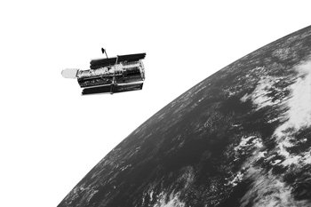
Perhaps the best-known orbiting observatory is the Hubble Space Telescope (HST). The HST is able to observe the visible and near UV. While most of these wavelengths can be studied from the ground, the HST was placed in orbit to avoid the blurring effects of the earth’s atmosphere. As starlight passes through the atmosphere, changing densities due to temperature changes cause the light to follow slightly different paths. The rapidly changing light paths make stars twinkle. Twinkling leads to blurred images. Large telescopes can never realize their full image-making ability because of this blurring. Above the earth’s atmosphere the HST has no problem with atmospheric blurring, so it has unparalleled resolution.
Telescopes
The heart of a telescope is its light-gathering device, which is called the objective. If the objective is a convex lens, the telescope is called a refractor, because the lens bends, or refracts, light to form an image. The other type of telescope is the reflector, so called because it uses a concave mirror that reflects light to form the image. The important functions of the objective are to collect light and form an image. The size of a telescope is defined by the diameter of the objective. For instance, a 60 mm telescope has an objective that is 60 mm in diameter. The HST has an objective that is 2.4 meters. The largest optical telescopes are the twin 10-meter Keck telescopes at the Mauna Kea Observatory in Hawaii.
Image courtesy of Bryan Miller
What are the advantages of a larger telescope? One advantage is that larger telescopes, having more objective surface area, gather more light. More light causes images to appear brighter. Distant objects too faint to be seen with a smaller telescope may be visible in larger telescopes. Since the observed brightness of an object decreases with distance, this means that larger telescopes allow us to study ever more distant objects. Another advantage of larger telescopes is that they produce more resolution. Resolution is the ability to see fine detail. This is especially noticeable with the planets. A larger telescope usually will show features that will not be visible in smaller telescopes. However, the previously mentioned blurring effect of the earth’s atmosphere limits this.
The distance between a telescope objective and the image of a far away object is called the focal length. We may examine the image formed by the objective by magnifying the image with an ocular, or eyepiece. The amount of magnification, or power, is determined by dividing the focal length of the objective by the focal length of the eyepiece. For example, an eyepiece with a 20 mm focal length used with a telescope with a 1,000 mm focal length will produce a magnification of 50 times. That is, objects viewed will appear 50 times larger. This is usually expressed as 50x.
The amount of magnification of a telescope is often over-emphasized in advertisements. As magnification is increased, the image does get larger, but the amount of the collected light is not increased. A larger image means that the available light is spread over a greater area so that the image appears much fainter than at lower power. In addition, any blurring caused by the earth’s atmosphere or imperfections in the optics will be greatly magnified by high powers. Therefore there is a limit to how much one may usefully magnify an image. A good rule is that the maximum magnification on the best nights should be no more than about 50x for each inch of diameter of objective. For instance, the highest power that one should ever use with a ten-inch telescope would be 500x. That would be the limit on the very best nights; on most nights less magnification should be used.
Professional astronomers spend little time peering through an eyepiece. Instead, equipment is attached to the telescope to measure and record the light. Sometimes the telescope is used as a camera lens to record an image. Once this was done with photographic emulsions, but the Charge Coupled Device (CCD) has largely replaced photography. A CCD is a computer chip with many small light sensitive elements that acquire charges proportional to the amount of light that falls upon them. To produce an image, a computer periodically reads the charges from the CCD. A CCD collects light much more efficiently than regular photographs can. Therefore, CCDs are much faster than photography, so that a one-minute CCD image can record as much light as a one-hour photograph. The studies of images can reveal much about celestial objects.
Photometry
Besides direct imaging there are two other primary uses of telescopes. One is photometry. The word photometry comes from two words that mean “light measure,” so photometry is the science of measuring light brightness. Many stars vary in brightness. Variable stars can change brightness for a number of reasons. Measurements of star brightness give us the raw data that permits us to determine why a particular star varies in brightness.
Astronomers use magnitudes to express star brightness. This system was developed by the Greek astronomer Hipparchus two millennia ago. There are two peculiarities with the magnitude system. One is that the smaller numbers correspond to the brighter stars, while the higher numbers correspond to the fainter stars. The brightest stars in our sky are first magnitude, while the faintest visible to the unaided eye on a dark night are about sixth magnitude. The faintest objects detectable today are fainter than magnitude 30. The full moon is about -12.5 magnitude and the sun is -26.8. The other peculiarity is that the scale is logarithmic. The system is arranged so that each difference of one magnitude corresponds to a factor of about 2.5 in brightness. A difference of five magnitudes is defined to be a factor of exactly 100 in brightness.
As an example, consider a first magnitude and a sixth magnitude star. First magnitude stars are roughly the brightest stars in our sky, while sixth magnitude is the limit of what the naked eye can see on a clear, dark night. A sixth magnitude star is five magnitudes fainter than a first magnitude star. Therefore the sixth magnitude star is 100 times fainter. How many times fainter than a first magnitude star is an eleventh magnitude star? This is a difference of ten magnitudes. Since this is a difference of five magnitudes twice, some might erroneously conclude that the stars differ in brightness by 100 + 100 = 200. However, each magnitude difference of five is a multiplicative factor of 100. Therefore a ten-magnitude difference is a factor of 100 x 100 = 10,000 = 104 . Similarly a fifteen-magnitude difference is a factor of 1,000,000 = 106.
What we have described thus far is apparent magnitude, how bright a star appears to us. However, a star’s brightness depends upon two factors: how bright it actually is, and how far away the star is. In professional circles stellar distances are usually expressed in parsecs, a unit that will be described later. Most people are more familiar with light years; a parsec contains 3.26 light years. If a star’s distance and apparent magnitude are known, then we can express the star’s actual brightness as an absolute magnitude. Absolute magnitude is defined as the apparent magnitude that a star would have if it were 10 parsecs, or 32.6 light years, away. The sun has an absolute magnitude of 4.8. Let m be the apparent magnitude, M the absolute magnitude, and d be the distance expressed in parsecs. The these quantities are related through the equation d = 10(m – M +5)/5 .
Spectroscopy
A third use of a telescope is spectroscopy. A prism or diffraction grating disperses light, which means that the light is broken up into a spectrum of different wavelengths. A device attached to a telescope that does this is called a spectrograph, and a record of a spectrum is called a spectrogram. Studying stellar spectra can tell us much information about stars. These include things such as temperature, size, composition, and motion.
Image courtesy of Bryan Miller
The simplest atom is that of hydrogen, which has a single electron orbiting the nucleus that usually contains one proton. Below is an illustration of a hydrogen atom. Notice that the electron can be found in one of a number of orbits. Each orbit is distinguished by a number designated as n, with n having positive integer values starting with one. The lowest orbit closest to the nucleus is designated n = 1, the next highest is designated n = 2, and so forth. As n increases in value, the orbits get closer together. For large values of the number n the orbits cram together toward a limiting maximum orbit size corresponding to a value of n approaching infinity. This limit of the orbit size amounts to the maximum size of the hydrogen atom.
Image courtesy of Bryan Miller
Hydrogen atom
Electron orbits are quantized. This means that electrons can be found only in orbits corresponding to an integer value of n as shown in the figure. An electron may not orbit part way between two orbits. Each orbit corresponds to some energy, with the innermost orbits having the least energy and the outermost having the most energy. Since the orbits are quantized, the energy of the electron is quantized as well. An electron can make a leap, or transition, from one orbit to another orbit. As an electron makes an upward transition from a lower to a higher orbit, it must gain energy. As an electron makes a downward transition from a higher to a lower state it must shed energy. One way that an electron can gain or lose energy is by the absorption or emission of a photon. Earlier in our discussion we found that the energy of a photon is directly proportional to the frequency of the photon. The greater the energy difference between two orbits, the greater the frequency of the photon involved.
Emission Spectra
Suppose that an electron in a hydrogen atom is in the n = 3 orbit. The electron can make the downward transition to either the n = 1 or n = 2 state. Since these downward transitions emit a photon rather than absorb one, these transitions happen quite easily. Another way of looking at this is to realize that the electron is going from a higher energy state to a level of less energy. This is the natural direction of processes, as dictated by the second law of thermodynamics. Often the electron will make the transition from the n = 3 to the n = 2 state, with the emission of a photon having an energy equal to the energy difference between the second and third orbits. The energy of this photon corresponds to a frequency in the red part of the spectrum. This transition and the resulting red photon are called H.
Suppose that instead of starting in the n = 3 state, the electron started from the n = 4 state. The electron would then have the choices of falling to the n = 1, 2, or 3 state. Suppose that the electron again went to the n = 2 state. Since the n = 4 orbit has more initial energy than the n = 3 state, the emitted photon must have more energy than the H photon. The greater energy results in a higher frequency, and the color of this emitted photon is more toward the blue end of the spectrum than the H. Actually, it does appear blue. This emission is called H.
Now suppose that the electron was initially in the next higher state of n = 5. If the electron made the transition to the n = 2 state as before, the energy difference would be greater still and the frequency of the emitted photon would be even greater. This photon is in the violet portion of the spectrum, and is called H. This series can continue indefinitely with ever-higher initial orbits with successive Greek letters. The energy differences become less and less with higher terms, so that the frequencies of the photons get closer together. This series is called the Balmer series, after the German physicist by that name who discovered it experimentally in the latter part of the 19th century.
The Balmer series was an important bit of information that guided Neils Bohr to devise his model of the atom around 1914. This model, while a little naive, is the basic model of the atom that we have today, and is the version of the modern theory that most of us are taught in school. There are additional series resulting from other transitions in the hydrogen atom. For instance, the Lyman series is in the UV and results from transitions to the n = 1 state from higher levels. The Paschen series is the result of transitions between the n = 3 level and higher states, but it is in the IR. All of these other series lie outside of the visible part of the spectrum, so only the Balmer series may be readily observed by humans. Indeed, even in the Balmer series only the first three emission lines are visible. All subsequent lines beyond H lie in the UV beyond what the eye can see, though they may be photographed.
How do electrons get into the higher energy states to begin with? Electrons can be elevated to the higher orbits by inputting energy, such as by heating or electrical discharge. Electrical discharge is used in low-pressure lamps. Examples of low-pressure lamps include many streetlights and fluorescent lights. As the electrons fall to lower energy states they emit photons only at discrete energies as just described. Therefore the spectrum emitted will be dark except at those wavelengths where emission occurs. Such a spectrum is called a bright-line, or emission, spectrum because the spectrum will have bright emission lines in it. Hydrogen produces a geometric progression of three spectral lines at the frequencies (or alternately, wavelengths) in the visible part of the spectrum as just described.
In like fashion other elements produce sets of spectral lines. However, since the energy differences between states are not the same, the photon wavelengths and patterns are different. The result is that every element has a unique set of lines. This is the basis of chemical analysis using spectroscopy. If a sample is heated or excited to fluorescence, a spectrogram of the emission will show the lines of the elements present. Emission spectra result from hot gases at low pressure. Emission lines as just described are seen in the spectra of nebulae and the chromosphere, an upper layer in the sun’s atmosphere.
Absorption Spectra
Most stellar spectra are very different from emission spectra. A hot solid, liquid, or gas at high pressure produces continuous spectra, where all wavelengths or colors are seen without any lines. If the light from a continuous source passes through a cooler, low-pressure gas, an absorption spectrum is seen. Absorption spectra have bright backgrounds interrupted by dark absorption lines. Another name for an absorption spectrum is a dark-line spectrum. The interiors of stars are hot, high-pressure gases, so they produce continuous spectra. The outermost layers of stars (the stars’ atmospheres) are cooler and less dense than the interior, so the resultant stellar spectra have absorption lines.
How do absorption lines form? The process is the reverse of that with emission lines. The electrons are initially in a lower state. If a photon having the correct amount of energy passes by, the electron can absorb the photon and use the photon’s energy to make the transition to a higher orbit. Eventually the electron will emit another photon and fall back to a lower state, but the new photon will generally have a random direction so that there is a net loss of photons in the original direction of motion of the light (outward from the star’s interior). For instance, electrons in hydrogen atoms initially in the n = 2 state can absorb photons having sufficient energy to elevate the electrons to the n = 3, 4, or 5 states. The amount of energy absorbed in each of these transitions is the same as when emission occurs. Therefore the wavelengths (or frequencies) of the photons involved will be identical to those as seen in emission. Thus an absorption spectrum is like a negative of an emission spectrum. Other elements have absorption lines at the same wavelengths as their emission lines as well. The spectra of nearly all stars are absorption spectra. A few strange stars, called Wolf-Rayet stars, have emission spectra instead.
When the spectra of various stars are compared, it is obvious that there is a bewildering array of different spectral lines in different stars. To make sense of this mess, about a century ago Harvard College Observatory began a program of classifying stellar spectra. The system that eventually emerged was one based upon temperature. In order of decreasing temperature, the spectral types are O, B, A, F, G, K, and M. Each class is subdivided into 10 subclasses that run from 0 to 9. The sun has spectral type G2. A slightly hotter star would be a G1 subclass, while a slightly cooler one would be G3.
Stars of spectral type A have the most intense Balmer lines of hydrogen, while O and M types lack Balmer lines. In G-type stars like the sun, the Balmer lines are moderately weak. One might expect that the presence or absence of the spectral lines of a particular element would signal the presence or absence of the element itself, but this is not the case. The weakness of Balmer lines of hydrogen does not mean that hydrogen is uncommon in the sun or that the absence of Balmer lines in O and M type stars means that those stars lack hydrogen. In fact, hydrogen is believed to be the most common element in nearly all stars. For spectral lines of a particular element to be visible, the element obviously must be present, but the electrons must be in the correct initial orbits as well. In absorption the Balmer lines require that electrons initially be in the n = 2 state. At low temperatures most electrons will be in the ground, or n = 1, state. Therefore, if the temperature of a star is too cool, most of the electrons will be in the lowest state and thus will be unable to make a transition that will produce a Balmer photon. If a star is too hot, nearly all of the electrons will be in highly excited orbits or even ionized. Therefore there will be too few electrons in the n = 2 orbit to produce Balmer lines. In summation, hydrogen Balmer lines can exist in stars only having a certain temperature range. The peak of the Balmer lines, where the largest percentage of hydrogen atoms have their electrons in the n = 2 state, is at a temperature of about 10,000°K. This temperature corresponds to the A0 spectral type.
The basic spectral types are a function of temperature, not composition..
Other elements have similar constraints on their visibility. The hottest stars (spectral type O) have atmospheric temperatures of about 40,000°K, and the only lines in their spectra are due to ionized helium. Less hot stars have neutral helium lines and weak hydrogen lines. At cooler temperatures the hydrogen lines strengthen while the helium lines fade. The hydrogen lines reach a maximum in the A type. Progressing to cooler types, the hydrogen lines gradually fade and are replaced by ionized metal lines. By the time the coolest stars are reached (spectral type M with temperatures of about 3,000°K), neutral metal lines and bands due to some molecules are present. In conclusion, the basic spectral types are a function of temperature, not composition.
However, there are a few stars (less than 1%) that do have odd compositions that render their spectra very different from the vast majority of stars. A striking example is the group of stars called carbon stars. As the name suggests, carbon stars contain much carbon. Typically stars have more oxygen than carbon, but carbon is more abundant in carbon stars. In normal red-giant stars all of the carbon is used up in forming carbon monoxide (CO), leaving the oxygen to combine with metals to form metal oxides that dominate their spectra. In carbon stars all of the oxygen is used up, leaving the carbon to form various carbon compounds. These compounds and free metals in the atmospheres of carbon stars change the atmospheric structure of carbon stars. This makes them very different from normal red giants. One obvious difference is that carbon stars are often far redder than normal red-giant stars. Carbon stars have been classified as R or N types that parallel the K and M types in temperature. A more modern classification combines the R and N types into a single C class.
Related to carbon stars are the metal stars, classed as S type. Metal stars have odd metal abundances. For instance, some S stars contain the element technetium, of which there are no stable isotopes. There are other examples of stars with odd spectra, but usually they can be grouped with more “normal” spectral types with various appended letters to indicate their peculiarities. For instance, some stars are appended with an “e” to indicate emission or an “m” to indicate magnetic fields. Astronomers have developed evolutionary theories to explain how these odd stars became this way.
Temperatures can be determined by spectral type, but there are other ways, as well. One method is by measuring color. Color is a result of a difference in magnitude measured at different wavelengths. Astronomers have devised filters that allow us to measure different parts of the spectrum. Two of the most common are the B filter that is in the blue part of the spectrum and the V filter that is in the visual (yellow-green) part of the spectrum. Except for their absorption lines, the spectra of stars greatly resemble the spectra of blackbodies. A blackbody is an object that perfectly absorbs and radiates electromagnetic energy. They are called blackbodies because at lower temperatures, such as room temperature, they appear black. Obviously at high temperatures they appear bright.
The illustration below shows a comparison of the spectra of two blackbodies having different temperatures. Notice that the curve of the hotter temperature is higher than that of the cooler temperature. Also notice that the peak of the hotter curve is at a shorter wavelength than that of the cooler curve. To the eye, a hot star appears blue, while a cool star appears red. Intermediate temperature stars appear yellow, with various shades in between. The B filter is so situated that it is near the wavelength where the spectrum of a hot star peaks, while the V filter is far from the peak. Therefore if magnitudes measured in either filter are compared, the B magnitude will be much brighter. However, for a cooler star the peak is nearer the V filter, and the B filter will be far from the peak. Therefore the V magnitude of a cooler star will be greater than the B magnitude. Since the magnitudes of a single star are what are being compared, the overall height of the curve is immaterial.
As a blackbody heats, the wavelength of maximum emission shortens and energy radiated increases at all wavelengths.
The magnitude difference is called a color index and is usually expressed as B-V. A very hot star might have a B-V of –0.10, while a very cool star might have a B-V of +1.70. The former star would appear blue and the latter would appear red. The sun is a yellow appearing, medium temperature star with a temperature a little less than 6,000°K. The B-V of the sun is about +0.62. This system of color index has been calibrated with accurate spectral types and generally offers a very efficient way to measure stellar temperatures.
Stellar Velocity
Spectroscopic data can tell us how fast stars are moving toward or away from us by the Doppler shift. As discussed in chapter 3, Doppler shift and cosmological redshift are not the same thing, though they appear the same. If a star is moving away from us, the lines in its spectrum will be shifted to longer wavelengths, while a star moving toward us will have its lines shifted toward shorter wavelengths. Many spectrographs can produce a laboratory spectrum of some material that can be recorded along with stellar spectra. We can calibrate the stellar spectra by comparing the laboratory and stellar spectra. Even small spectral shifts caused by motion of only a few kilometers per second can be measured this way. The only motions that spectroscopy can measure are those in the line of sight; transverse motion perpendicular to the line of sight cannot be measured this way. Line-of-sight motion is called radial velocity, while transverse motion is called tangential velocity.
Radial velocities are very helpful. For one thing, it is a direct confirmation that the earth moves around the sun. Our orbit around the sun causes the radial velocity of most stars to shift in a sinusoidal fashion throughout the year. That is, stars lying near the earth’s orbit around the sun have their radial motions vary by plus and minus 30 km/sec each year. That speed is the rate at which the earth orbits the sun. Therefore radial velocity measurements must be corrected for this effect to express radial velocities with respect to the solar system. Since the sun is the center of the solar system, measured radial velocities corrected for the earth’s motion around the sun are called heliocentric radial velocities. Heliocentric radial velocities tell us which stars are moving toward the sun and which are moving away, though the measured radial velocity is actually a combination of a star’s motion and the motion of the sun. Analysis of radial velocities of a huge number of stars has enabled astronomers to determine what is called the local standard of rest. We also know that the sun is moving around the center of the galaxy at a speed of about 250 km/sec. This information allows us to estimate the mass of the galaxy.
Radial velocity measurements are very important in the study of binary stars. A binary star is a system of two stars that are orbiting around each other by their mutual gravity. As the members of a binary star orbit each other, they may alternately move toward and away from us, resulting in periodic Doppler shifts in the spectral lines. These shifts allow us to model the system and determine basic stellar parameters, such as mass. Close binary stars are the sites of many interesting astronomical phenomena. For instance, many close binary stars have mass transfer from one star to the other, a process that is readily observable with spectroscopy.
In recent years these kinds of radial velocities have been used to search for extra-solar planets, that is, planets orbiting other stars.1 In a binary-star system, both stars move because either star pulls on the other with its gravity. Newton’s third law of motion ensures that the amount of force on either is equal in magnitude. How much either star moves depends upon how similar their masses are. If the masses are equal, then the stars will move equally. If one star has more mass than the other, then the less massive star will move more, with the ratios of the stars’ motions inversely proportional to the masses of the stars. In fact, this relationship is what allows us to determine the masses of stars in binary-star systems. Planets also move the sun, but because the sun has so much more mass than the planets, the planets do almost all of the moving while the sun does very little. The search for extra-solar planets relies upon looking for very subtle Doppler shifts in the candidate stars. A small periodic shift in a star’s spectrum could be evidence of a planet orbiting that star. When one calculates the amount of mass required to produce these subtle orbital motions in a star and finds that the mass is far too small to be a star, then we are left with the conclusion that the unseen orbiting body must be a planet. Most astronomers agree that we have found many extra-solar planets, with the list growing.
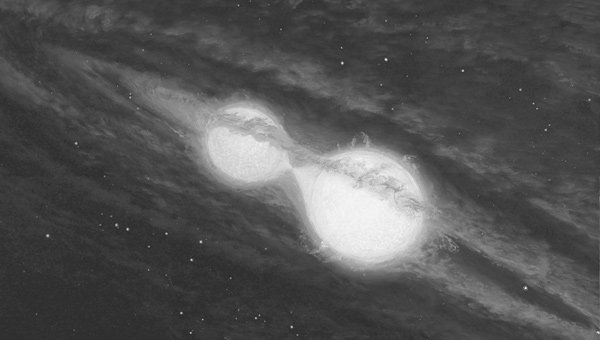
Image courtesy of Science Photo Library
Artist’s concept of a binary star system
The observation of extra-solar planets is not without controversy. Even single stars may exhibit periodic radial velocities. Many variable stars are pulsating. That is, they regularly expand and contract. As these stars expand and contract they alternately produce radial velocities toward and away from us that are superimposed upon their regular motion. As these stars expand and contract, their temperatures also change. You should recall that as a gas expands it cools, and as it is compressed it heats. The complex interplay of changing size and temperature causes pulsating stars to noticeably change in brightness. This is what makes them variable stars. The very subtle periodic Doppler shifts in the candidate hosts of extra-solar planets are orders of magnitude lower than those of pulsating stars. Therefore some astronomers at first suggest that if the stars that allegedly host other planets are actually pulsating, then the small changes in the sizes of these stars might not be readily visible as light changes. This objection has been overcome to the satisfaction of most, and so this does not seem to be a way of explaining away the existence of extra-solar planets.
As an aside, is the existence of other planets a problem for the biblical world view? Not really. Most creationists assume (rightly so, I believe) that there is no life on other planets (extraterrestrial life). Some creationists apparently think that denying that there are other planets will somehow limit this possibility. However, we should welcome other planets. All of the planets discovered at the time of the writing of this book are obviously hostile to any form of life, because most are too massive or too close to their parent stars, or both. This should be a powerful witness to us that our planet is special. Even if some of these planets might be hospitable to life, we know that life from non-living matter apart from creation is impossible.
Tangential velocities are much more difficult to measure than radial velocities. Motion in the tangential direction results in a gradual change of a star’s position in the sky. Comparison of photographs of stars made many years apart tell us how fast stars are changing position. The average annual change in position of a star is called the star’s proper motion and is expressed in arc seconds per year. Most proper motions are very small. The largest proper motion is that of Barnard’s Star which is only 11.2”/yr. Barnard’s Star takes about 160 years to move the equivalent diameter of the moon. Proper motion depends both upon the tangential velocity and the distance. A star that is moving very rapidly in the tangential direction must not have a large proper motion if it is far away. Conversely, a star that is nearby may have a large proper motion but a modest tangential velocity. In order to find the tangential velocity, we must know both the proper motion and the distance. Generally the nearer stars have the larger, and hence more accurately known, proper motions. We also know the distances of nearby stars better. Therefore the measurement of tangential velocities is restricted to the nearer stars, while radial velocities may be found for any distance.
Stellar Mass
The masses of stars are found by the study of binary stars. As stated above, the members of binary-star systems orbit by their mutual gravity. For a given separation, the orbital speed and period depend upon how much gravity is present. The amount of gravity in turn depends upon the amount of mass. The masses of hundreds of stars have been determined this way. The least massive stars are about 8% that of the sun, and the most massive are a few tens of times the mass of the sun. While we can find the masses of stars only in binary systems, we find in binary systems a wide range of stars that appear otherwise identical to solitary stars. Therefore it is reasonable to conclude that we know the masses of stars with confidence.
Astronomers have measured the mass of the galaxy by treating the sun and the galaxy as a binary-star system. As mentioned above, the sun is orbiting the galaxy with a speed of about 250 km/sec. We think that the sun is about 25,000 light years from the center. It is simple physics to calculate the acceleration and hence the mass necessary to keep the sun in orbit. The amount of mass is about 1011 solar masses. Similar studies of other objects orbiting our galaxy and other galaxies have indicated that dark matter may exist.
Stellar Size
Eclipsing binary stars offer us a direct way of measuring the diameters of stars. An eclipsing binary is a binary in which the orbital plane is viewed nearly edge-on so that with every orbit the stars pass in front of, or eclipse, each other. Obviously, larger stars take longer to eclipse each other than smaller ones do, so the duration of the eclipses tell us how large the stars are. Perhaps hundreds of stars have had their sizes measured this way. When similar stars from different eclipsing binaries are compared, their sizes agree pretty well. This gives us confidence that when we see other stars that are not in eclipsing binary systems, but are otherwise similar to ones that are, then we probably know the sizes of those stars as well.
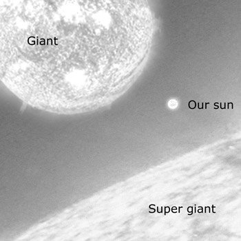
This illustration shows the difference in the size of our sun compared to the largest stars.
There are several indirect ways of finding the sizes of stars. From time to time the moon passes in front of a star, which is an event called an occultation. Both the star’s disappearance behind the moon and its later reappearance on the other side happen very quickly (usually far less than a second). High-speed photometric measurements reveal that the star does not disappear instantaneously, but “gradually” over a tiny fraction of a second. Often this takes thousandths of a second. The rate at which the star disappears and later reappears depends upon several things such as the speed of the moon in its orbit, the angle that the edge of the moon makes with the moon’s motion, and the apparent size of the star. The apparent size is the angle subtended by the star, and is usually expressed in units of milli arc seconds, or thousands of a second of arc. All other factors are known, so from the data we can calculate how large the angular diameter is. However, we can convert the angular diameter to actual linear diameter (in kilometers) only if we know the distance to the star. This is why this is an indirect method. If the distance is not known, then the star’s diameter cannot be found.
While the lunar occultation method works very well, the moon occults stars only found in a swath about 11 degrees wide centered along the ecliptic. Most stars are not found in this narrow region of the sky. Interferometry was discussed briefly in chapter 1. It is the technique of using the principle of interference resulting from the wave nature of light to glean certain information from the light. This can be done with the light of some stars to measure their angular diameters. As with the lunar occultation method, the distance of the star must be known to find the actual diameter, so this too is an indirect method. It also suffers from the limitation that only stars with very large angular diameters can be measured, so it is restricted to much larger angular diameter stars than the lunar occultation method.
A fourth method of finding stellar diameters involves using some well-understood physics. The Stefan-Boltzmann law states that the amount of energy given off by a blackbody goes at the fourth power of the temperature. In equation form, L = σT4 where L is the luminosity (the total energy radiated per second), T is the temperature in Kelvin, and σ is a physical constant. The total brightness of a star also depends upon the surface area of the star. Stars are generally spherical, so the area should be 4πR2. These two equations can be combined into a single equation, but the units will be a bit cumbersome. Therefore, astronomers usually change to solar units to simplify the equation: L = R2T4 where L, R, and T are the luminosity, radius, and temperature of a star expressed in solar units. What are solar units? They are the quantities in terms of the sun’s units. For instance, the sun’s luminosity is 3.88 x 1033 erg/sec, so that amount is defined to be one. The sun’s radius is 6.96 x 1010 cm, so that is the unit of radii. The sun’s surface temperature is 5,770°K, so that is one unit of temperature.
This equation can be turned around to solve for R, but first we must know T and L. The determination of temperature is straightforward by spectral type of color as previously discussed. Luminosity is more difficult. We must know the distance to convert the apparent magnitude to absolute magnitude. Inverting an earlier equation that related these quantities can do this. However, both apparent and absolute magnitudes are measured at certain wavelengths, such as in the B or V filters. The luminosity must be expressed as the power released by a star when all wavelengths are considered. Such a magnitude is called the absolute bolometric magnitude. It is not possible to measure bolometric magnitudes, so we calculate them using what measurements we can and stitching together the rest of the spectrum and well-understood physics. Some astronomers have spent much of their professional careers preparing tables for other astronomers to make these transformations. Once an absolute bolometric magnitude has been found, we can easily convert this to luminosity to put in the equation.
Since this method of finding stellar sizes is not limited to stars along the ecliptic, it is very powerful. However, since it requires knowing the distance of each star measured, it is an indirect method. It is also dependent upon certain models, such as stellar-atmospheric models that permit the conversion of an observed magnitude into luminosity. This introduces error, but there are limits on that error. It is probable that we can determine sizes of stars by this method to within 20%.
Finding Stellar Distances
There is only one direct method of finding stellar distance—trigonometric parallax. In the introduction we found that parallax is the apparent shift of a star as the earth orbits the sun each year. The illustration below shows a diagram of how trigonometric parallax occurs. Notice that there is a very thin triangle with the small angle at a star. This angle is called the parallax angle, and is usually designated by the letter π. Here π is a variable, not the constant defined to be the ratio of a circle’s circumference to its radius and approximated by 3.14. One leg of the triangle is the line between the star and the sun, and the other leg is the line between the star and the earth. The base of the triangle is the line between the earth and sun. The base has a length of one astronomical unit (AU). The length of either of the two legs is the distance to the star, d. Since the parallax angle is so small, we can use the small angle approximation, π = 1/d
Image courtesy of Bryan Miller
Trigonometric parallax
In conventional units, the parallax would be measured in radians and the distance would be expressed in AU. Since stars are so far away, all parallax angles would be very tiny and distances would be very large when expressed in the conventional units. Therefore, astronomers use their own units. Parallax angle is measured in seconds of arc, and so a new unit of distance must be defined. The new unit is defined to have a value of one when the parallax is one second of arc. We define this unit to be the parsec (pronounced par-seck, and abbreviated pc) from parallax of one second of arc. A parsec is equal to 3.26 light years. The closest star, α Centauri, has a parallax of 0.76 arc seconds, so its distance is about 1.3 parsecs.
The first parallax was measured in the 1830s, and for 160 years all parallax measurements were done in pretty much the same way. The classical techniques from the ground have errors of about 0.01 arc second. Since this error amounts to a parallax of 100 pc, many people mistakenly conclude that measurements by these methods will yield distances out to about 100 pc (or about 300 light years). However, when the error is the same size as the measurement, we cannot be sure that we are measuring any parallax at all. Classical measurements can produce distances within 20% accuracy only to about 20 pc (65 light years).
During the 1990s several new techniques were pioneered to measure more accurate parallax. The most successful of these was the HIPPARCOS satellite launched by the European Space Agency. The HIPPARCOS mission measured the distances of several hundred thousand stars, with an accuracy that exceeds that of classical techniques by an order of a magnitude. We now know the distances of stars to nearly 200 pc, about 600 light years. The importance of the HIPPARCOS results is that they allow calibration of other, indirect methods.
There are other methods of finding stellar distances, though those methods are not as important as they were before HIPPARCOS. We will discuss two related methods. We have previously mentioned pulsating variable stars. Pulsating variables regularly repeat their light variations over an interval called the period. If we plot measured magnitudes over the period, we get what is called a light curve. The average magnitude is the average of the maximum and minimum magnitudes. Pulsating stars have distinctive light curves that are usually marked by a rapid rise to maximum light followed by a more gradual decline toward minimum light.
One class of pulsating stars, the RR Lyrae stars, appear to be very similar to one another. They vary by less than a magnitude, and they have periods of oscillation of a few hours up to less than a day. Their most important feature is that they all have about the same absolute average magnitude, 0.6. RR Lyrae stars are easy to identify by their light curves, and once we realize that they have the same absolute average magnitude, and then we can use their observed average magnitude to find their distances. RR Lyrae stars are very common in a kind of star cluster called a globular cluster, so they are very useful in determining the distances of globular clusters.
Similar to the RR Lyrae stars, but much larger and brighter, are the Cepheid variables. Cepheid variables are giant and super-giant stars that have periods of anywhere from a few days to more than 50 days. They can vary over a few magnitudes. Early in the 20th century the astronomer Henrietta Leavitt discovered that the period of a Cepheid variable is directly related to the average absolute magnitude. That is, the brighter that a Cepheid is, the longer that it takes for the star to vary. A calibrated plot of this relationship is called the period-luminosity relation. From a Cepheid’s light curve we can read off its period. The period-luminosity relation gives us the absolute average magnitude. The average magnitude of the light curve is the average-apparent magnitude. The distance can be found as before.
Since both RR Lyrae and Cepheid variables may be seen much farther than the 600-light-year limit of trigonometric parallax, they allow us the find distances beyond what parallax can produce. However, the RR Lyrae and Cepheid variable methods of finding distances are indirect in that they rely upon the assumption of the constancy of the average RR Lyrae magnitudes and the validity of the period-luminosity relation of Cepheids. Both of these assumptions appear warranted from observations. All the other methods of finding distances rely upon similar sorts of assumptions, often based upon some well-accepted physics. The result is that stellar distances are probably known to a few hundred or even thousand light years with great confidence.
Extra-Galactic Distances
Most methods of finding stellar distances apply only to stars within our own galaxy, the Milky Way. However, many of these methods also work on two small satellite galaxies of the Milky Way, the Large and Small Magellanic Clouds. They are about 160,000 light years away. Beyond these systems the only method of stellar distance that works is the Cepheid variables. This method works for galaxies out to a few tens of millions of years because Cepheid variables are so bright. Generally when we talk about distances of other galaxies, we must develop other methods based upon “standard candles.” A standard candle is a bright object for which we think that we know how bright it is, or in other words, we know its absolute magnitude. Examples of standard candles include bright globular clusters, HII (pronounced H-2) regions, super-giant stars, novae, and type Ia supernovae.
There are about 200 globular clusters in the Milky Way Galaxy. Since RR Lyrae stars are common in globular clusters, we have a good idea of how far away most of them are. Knowing their distances we can estimate how bright each cluster is and how large each cluster is by how bright and how large each cluster appears to us. Astronomers have found that globular clusters in our galaxy do not have a large range in size or brightness. The biggest and brightest are surprisingly uniform. Assuming that globular clusters in other galaxies similar to the Milky Way follow similar trends, we can estimate the distances of those other galaxies by how large and bright their globular clusters appear.
HII regions are clouds of glowing gas excited by the UV photons given off by bright, hot stars in their midst. There are many HII regions in the Milky Way and other similar galaxies. While there is a greater range in HII-region brightness and size than with globular clusters, the largest and brightest ones appear to be uniform from galaxy to galaxy. This uniformity allows us to treat the largest and brightest HII regions as standard candles.
Within a given galaxy of perhaps 200 billion stars, there will be a few dozen extremely bright stars. These are super-giant stars and represent the brightest stars of all. From galaxy to galaxy these bright super giants appear to have about the same absolute magnitude, so they too represent a standard candle. From time to time within galaxies there are novae (novae is plural, the singular is nova), stars that abruptly flare up in an eruption that lasts a few days. Astronomers think that novae are the result of material transferring from one star to another in a particular kind of binary-star system. The brightest novae all appear to have the about the same absolute magnitude, so they can be used as a standard candle as well. All of the standard candles mentioned thus far have nearly the same absolute magnitude, about –9. Generally, if more than one of these methods is available, all of the distance measurements are averaged.
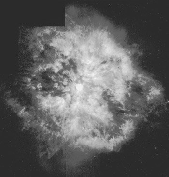
Image courtesy of NASA
Supernova remnant
A supernova is an extremely violent explosion of a star in which sometimes the precursor star is completely disrupted. A supernova may rival in brightness the galaxy in which it occurs. A supernova may remain near peak brightness for weeks before slowly fading over many months. There are two basic types of supernovae, type I and type II. The two types are markedly different in the types of light curves that they follow and the types of spectral lines that they have. A type II is the explosion of a very massive single star. Type II supernovae have considerable range in their peak brightness. Type I supernova result from mass transfer in close binary stars where the star that is gaining mass is a special kind of dense star, such as a white dwarf.
Of particular interest is a subset of type I supernovae, the type Ia. Type Ia supernovae have the same absolute magnitude near maximum light, about –19. Since we know the absolute magnitude of type Ia supernovae, we can use them to measure extremely large distances, often leap-frogging over other methods. A type Ia supernova occurs perhaps once or twice per century in any galaxy, so we can see a number of them per year in other galaxies. Type Ia supernovae have been used to measure distances of galaxies more than a billion light years away.
The Hubble relation was discussed in chapter 1, so it will not be further described here. To use the Hubble relation, the Hubble constant must be determined. We do this by measuring the distances of as many galaxies as possible, and comparing the distances to the measured redshifts. The greatest difficulty is that nearby galaxies have the best distances, but the lowest redshifts, while more distant galaxies have the poorest distances and the greatest redshifts. A redshift is comprised of two parts: a Doppler shift due to motion and a Hubble flow due to universal expansion. For nearby galaxies expansion is minimal, so Doppler motion tends to dominate the redshift. With increasing distance, Doppler motions do not change, but the Hubble flow increases. Ideally, we would like to use the most distant objects possible to calibrate the Hubble constant, because then any Doppler motion can be ignored. The problem is that we can best measure distances for nearby objects, while distant galaxies are difficult to measure. Most disagreement over the value of the Hubble constant centers on how to handle this problem. Since type Ia supernovae skip over large distances, they have become very important in finding the value of the Hubble constant. When all is said and done, we find that with some exceptions, distance does scale with redshift. The most plausible interpretation of this fact is that the universe is expanding.
In this appendix we have attempted to show how astronomers can determine basic stellar properties. Modern astronomy allows us to find the distances, sizes, temperatures, and masses of stars. This is incredible, given how far stars are from us.
Checking Your Understanding
- What are the two types of telescopes? How are they different?
- How do we determine the size of a telescope? What are the advantages of a larger telescope?
- What are two peculiarities of the magnitude system for measuring stellar brightness?
- What are the seven basic stellar spectral types? What factor is responsible for the various spectral types?
- What do we learn by studying binary stars?
- What is the only direct method for finding distances to stars? How far out can we measure stellar distances with this method today?
- Why can Cepheid variables be used to find distances?
- Why can type Ia supernovae be used to find distances?
Universe by Design
This book explores the universe, explaining its origins and discussing the historical development of cosmology from a creationist viewpoint.
Read Online Buy BookFootnotes
- Wayne Spencer, TJ.
Support the creation/gospel message by donating or getting involved!

Answers in Genesis is an apologetics ministry, dedicated to helping Christians defend their faith and proclaim the good news of Jesus Christ.
- Customer Service 800.778.3390
- Available Monday–Friday | 9 AM–5 PM ET
- © 2025 Answers in Genesis