
Research conducted by Answers in Genesis staff scientists or sponsored by Answers in Genesis is funded solely by supporters’ donations.
Abstract
The young-earth creation model currently lacks a robust explanation for molecular diversity. No comprehensive method exists by which absolute or relative sequence differences among species can be predicted, and no method has been formulated to rigorously predict the function of molecular residues, especially those in so-called “house-keeping” proteins. In this study, I derived a method to predict the function of molecular differences between biblical “kinds.” Applying this method to the mitochondrial “house-keeping” protein sequences of ~2700 species, I found that differences among “kinds” were not due to neutral changes since creation, but were explicable in functional terms. This finding has implications for the mechanisms and feasibility of species’ change. Conversely, I also found that absolute genetic differences within a “kind” were predictable to a first approximation by modern mutation rates and the young-earth timescale. These data provide a compelling alternative to old-earth and evolutionary explanations for molecular diversity, and they challenge the millions-of-years timescale common to these models.
Keywords: mitochondria, DNA, sequence alignment, young-earth, mutation rate
Introduction
Why do anatomically distinct species share molecular sequence? Why do morphologically similar species diverge at the genomic level? Reconciling these seemingly contradictory phenomena is the major task of origins molecular biology.
The creation and evolutionary models contrast sharply in their explanations of these facts. The evolutionary model explains these molecular patterns with a single rule: Species have diverged over millions of years from a universal common ancestor. Occasionally, evolutionists make an exception to this rule and appeal to convergent evolution, but their primary explanation is descent with modification. Specifically, evolutionists attribute the existence of shared sequences among diverse species to inheritance from a common ancestor. Conversely, they explain genetic distance as a function of evolutionary time—the more time that has elapsed since two species shared a common ancestor, the greater the molecular difference between them.
In support of these claims, evolutionists cite the nested hierarchical order among species’ molecular differences as evidence of their common ancestry through evolutionary time (Dawkins 2009; Theobald 2012). For example, they cite the genetic similarity among humans and chimpanzees as evidence of their recent common ancestry (within the last few million years) (Carroll 2005), and they explain the dramatic genomic structural differences among Drosophila species (Drosophila 12 Genomes Consortium 2007) as reflective of their more distant common ancestry (tens of millions of years) (debates over the precise human-chimpanzee sequence identity notwithstanding [Bergman and Tomkins 2012; The Chimpanzee Sequencing and Analysis Consortium 2005; Tomkins 2011; Tomkins 2013; Tomkins and Bergman 2012; Wood 2006a]).
The evolutionary model is so robust that it leads to predictions of molecular function. Under the assumptions of this model, species will grow more and more distant molecularly over time, unless some natural force constrains random variation. For proteins that have evolved differences rapidly, evolutionists predict that these proteins have fewer functional constraints than proteins which have evolved differences slowly (Futuyma 2009).
The evolutionary model also predicts that sequences which are highly conserved among distantly related species are functional. Natural selection is the only available mechanism under this model by which sequence identity can be maintained over time, and if two species that diverged early in evolution still share some level of sequence identity, natural selection must have preserved this commonality. Since natural selection requires a function upon which to act, shared sequences between these species must be functional.
In contrast, the creation model offers a very different explanation for molecular unity and diversity. Creationists explain shared sequences among diverse species either by God’s initial creation act or by convergence since the Creation week. In either scenario, the creation model—like the evolutionary model—predicts that highly similar sequences in different species exist for a functional purpose.
Unlike the evolutionary model, the creation model lacks a clear, predictive explanation for molecular diversity. Because Scripture is silent on the identity of the sequences that God created during the Creation week, a number of competing explanations still exist. For example, molecular differences between two individuals might be due to the initial creation of sequence differences between them, or to the accumulation of random changes since the Creation week. These contrasting explanations make opposite predictions about the function of the sequences in question. Data to date have not resolved the precise relationship between these explanations, and this ongoing ambiguity makes the creation model weak on the question of molecular diversity.
This conundrum intensifies when considering hierarchical sequence patterns. For example, different species of Drosophila are more genetically distant from one another (Drosophila 12 Genomes Consortium 2007) than humans and chimpanzees are from one another (again, debates over the precise sequence identity notwithstanding [Bergman and Tomkins 2012; The Chimpanzee Sequencing and Analysis Consortium 2005; Tomkins 2011; Tomkins 2013; Tomkins and Bergman 2012; Wood 2006a]). Yet, the Drosophila species likely share a common ancestor since they belong to the same biological family (Wood 2006a), whereas humans and chimpanzees clearly have separate ancestries (Genesis 1:26–28). Why would differences between the related species exceed differences between unrelated ones?
This puzzle becomes even more challenging when considering genes that are thought to perform the same vital function in very diverse creatures (i.e., “house-keeping” genes). For instance, the sequence for the house-keeping gene cytochrome c is more similar between humans and primates than between humans and insects. From a creation perspective, it is tempting to immediately invoke function as an explanation for these differences since humans share more anatomy and physiology with chimpanzees than with fruit flies. But what does cytochrome c have to do specifically with the shared features (e.g., with the presence of four limbs)? Furthermore, since many positions in protein sequences appear to be functionally redundant (McLaughlin et al. 2012), why do “house-keeping” genes have any sequence differences at all? This dilemma is so penetrating that evolutionists have exploited it in their criticism of the creation model (Theobald 2012).
Hence, the young-earth molecular biology model faces a daunting challenge: (1) Predict absolute sequence differences between different species; (2) predict the relative hierarchy of sequence differences among species; (3) predict molecular function for differences among species.
Biblical Constraints on Molecular Explanations
Any molecular model proposed in answer to these challenges must conform to the explicit teaching of Scripture. Several scriptural parameters restrict and inform potential explanations.
First, molecular diversity must be explicable on a relatively short timescale—several thousand years. This is seen clearly in Genesis 1 . The text describes a literal, six-day Creation week that includes the creation of biological organisms on Days 3, 5, and 6, and the date of this Creation week is around 6000 years ago according to the genealogies of Genesis 5, Genesis 11, Matthew 1, and Luke 3. The Creation week cannot have occurred more than 12,000 years ago (McGee 2012). Thus, any biblically consistent model of genetic differences must conform to a recent time frame (thousands, not millions, of years).
Second, genetic ancestry must ultimately trace back to the created “kinds” of the Creation week. Genesis 1 repeatedly uses the phrase “after their kind” to describe the biological results of God’s spoken activity, and in this context, this phrase suggests a grouping or type. These types were not predated by any other organisms; universal common ancestry is not the biblical model for molecular origins. Thus, modern molecular differences must not be traced back beyond the Creation week to “pre-creation” sequences.
Third, genetic ancestry must be limited to members of the same “kind.” On this parameter, the Flood account is clear. When God commanded Noah to take the air-breathing land animals on board the Ark, He commanded that at least one pair of every “kind” be preserved (Genesis 6:19–20). Why? “To keep seed [offspring] alive upon the face of all the earth” (Genesis 7:3; KJV). God could have commanded pairs of some of the land, air-breathing “kinds” to be brought on board the Ark. However, had He done so, this passage implies that the “seed” of those “kinds” not on board the Ark would have become extinct in the Flood. Phrased differently, if one “kind” of creature could be changed into another “kind” of creature, then there would be no need to take pairs of every “kind” on board the Ark. A few pairs would have sufficed to keep “seed” alive after the Flood. Since pairs of every “kind” were commanded, “kinds” cannot be changed into other “kinds,” and genetic ancestry for a species is limited to a single “kind.”
Finally, large amounts of genetic change within “kinds” are biblically permissible. In all 31 uses of the Hebrew word transliterated as min (translated in English as “kind”), Scripture never forbids intra-“kind” change. Hence, the genetic change within a “kind”—even change that leads to the formation of new species—is biblically compatible.
Hypotheses on Mitochondrial DNA Diversity
These biblical parameters lead to three major hypotheses for the origin of modern molecular differences among species’ house-keeping genes. First, God may have created sequence diversity among individuals when He created each “kind” and each member of each “kind” during the Creation week. Second, modern species’ sequences may be the result of non-random change processes since the Creation week. For example, designed mechanisms of change may have altered the original sequences, and natural selection may have produced non-random outcomes for a set of randomly changed sequences. Third, diversity may the outcome of strictly random change processes, random both on the mechanistic and outcome steps of the process.
Focusing the Explanatory Task: Mitochondrial DNA Origins
I explored and tested these hypotheses on the published metazoan mitochondrial DNA and protein sequence dataset. Metazoan mitochondrial genomes contain, as a general rule, a set of RNA-coding genes (tRNAs, etc.), sections of non-coding DNA sequence (e.g., the D-loop), and the same 13 protein-coding genes (see data presented in this paper). All 13 of the latter are identified as involved in the mitochondrial electron transport chain and would, therefore, be immediately classified as “house-keeping” since they appear to perform the same basal biochemical function of energy transformation in all metazoans. Yet, in these proteins, profound sequence differences exist across the animal kingdom (see data in this paper). Thus, this dataset provided a unique opportunity to identify and formulate a detailed creationist response to the evolutionary challenge stemming from the apparent functional redundancy of residues within “house-keeping” proteins (Theobald 2012).
This metazoan mitochondrial dataset also possessed practical advantages over other molecular datasets. At the time of this study, ~2700 metazoan species with completely sequenced mitochondrial genomes were present in the database, representing multiple phyla, classes, orders, and families. If family is used as the surrogate measure for the “kind” boundary (Wood 2006b), this database effectively contains a large diversity of biblical “kinds.” Thus, by using this dataset, I could test creationist hypotheses across numerous “kinds” simultaneously and thereby discover the general explanatory principles for the young-earth model rather than isolated cases. Conversely, by limiting the analysis to only mitochondrial sequences, I simplified the number of potential models of sequence change because mitochondrial genomes are thought to be inherited uniparentally in many, but not all, animals (Al Rawi et al. 2011; Sato and Sato 2011).
Together, these considerations suggested that comparison of metazoan mitochondrial sequences would be useful means of elucidating the details of the young-earth model of molecular diversity. For practical reasons that follow, I investigated diversity between “kinds” separately from diversity within “kinds.”
Explaining Molecular Diversity Between “Kinds”
What might be the explanation for mitochondrial sequence differences between animal “kinds”? Given the apparent “house-keeping” function for the mitochondrial protein-coding genes, it is tempting to speculate that mitochondrial genomes were created identical across all “kinds” and that they performed the identical function in each. Under this hypothesis, current molecular differences represent random changes since creation, largely unaffected by natural selection. In the absence of selection, modern differences due to random change would be functionally neutral.
In contrast, perhaps God created sequences unique to each “kind” for a functional molecular purpose (hitherto unknown). Given the complexity of intracellular interactions and function, God may have created even the individual members of each “kind” genetically distinct. Under this hypothesis, genetic differences between “kinds” are a product of three factors—(1) initial (created) diversity between “kinds”; (2) initial (created) diversity within “kinds”; and (3) time (for mutations to accumulate). Predicting function under the hypothesis of an identical starting sequence is less complicated than under this hypothesis, yet the latter clearly predicts more function for molecular differences than the former.
Testing Molecular Diversity Hypotheses
How might these (and other) hypotheses be tested? Ideally, any methods that were employed would reveal the original sequence that God created in each “kind.” For example, population genetic models might be constructed for each of these hypotheses, and the predictions of these models might be compared to modern molecular data. However, empirically determined mitochondrial mutation rates are critical to make these models realistic, and these rates are known for only four metazoan species (Denver et al. 2000; Haag-Liautard et al. 2008; Parsons et al. 1997; Xu et al. 2012). Hence, discovering the original Creation week sequence for all metazoan “kinds” seemed unfeasible with current data.
Alternatively, the functional predictions of each hypothesis might be tested as a surrogate for empirically determining the original mitochondrial genome sequence. The most straightforward method to test the functional component of each hypothesis is systematic mutagenesis—individually mutating each amino acid in each of the 13 proteins in each species. This would unambiguously answer the question of whether current amino acid differences between “kinds” represent neutral change over time, or functional change/functionally created diversity. However, the vast number of species and the sheer volume of individual sequence differences to examine (see data in this study) made this experiment cost and labor prohibitive.
A third method for testing these hypotheses is nuanced and somewhat counterintuitive, but powerful. Rather than test each hypothesis directly, a strict null hypothesis could be constructed and then refuted. This would necessarily imply that one of the alternatives to the null must be true. For example, elimination of the null might point towards created diversity as the likely candidate. Hence, by process of elimination, the real explanation might be discovered.
In this paper, I formulated and tested a null hypothesis for mitochondrial sequence diversity. This hypothesis consists of two claims: (1) God created all metazoan “kinds” with the same mitochondrial genomic sequence during the Creation week. This implies that all “kinds”—from giraffes to grasshoppers—had an identical mitochondrial sequence in the beginning, including each individual member of each “kind.” (2) All change since the Creation week has been random. This means that mechanisms such as natural selection and nonrandom means of mutation (e.g., site directed mutases such as the rag genes in the immune system) cannot be invoked to explain molecular differences. Essentially, claim #2 represents an infinite sites model where any site can be mutated at random without functional consequence.
On these two points—one common starting sequence and strictly random change over time— the null hypothesis resembles the evolutionary assumption of a single common ancestral sequence for mitochondrial DNA origins, but on a much shorter timescale and with stricter limits on ancestry.
Testing the Null Hypothesis
With respect to molecular diversity between separate “kinds,” the null hypothesis used in this paper makes very specific predictions. Since the null postulates that all “kinds” began with the same sequence and diverged randomly over time, the null predicts that all “kinds” will grow more distant over time. By definition, no mechanism exists under the null hypothesis that would keep “kinds” molecularly identical to one another or that would direct them to change along the same molecular path. Biblically speaking, “kinds” have separate genetic ancestries (see justification in “Biblical constraints” section), and natural selection and non-random mutation are both excluded by definition. No directionality to change is possible under the null.
This claim immediately presents a test by which the null can be refuted. If sequence comparisons between “kinds” show evidence of directional change, then the predictions of the null are violated, and the hypothesis must be false. When the null is violated, alternatives to the null must then be true—either God created sequence diversity among “kinds,” or change has happened non-randomly, or both. Any of these latter explanations would imply a functional role for the sequences compared.
A third explanation might also be true. God may have created genetic diversity simply for aesthetic reasons. However, testing this hypothesis is nearly impossible at the present. Furthermore, given the amount of function already demonstrated for individual nucleotides in the human genome (ENCODE Project Consortium 2012), this hypothesis seems unlikely. Information compression at the genomic level seems too great to invoke purely aesthetic reasons for the existence of certain nucleotides. While the functional interplay among nucleotides is certainly elegant and aesthetically pleasing, the complexity of molecular interactions argues against strictly aesthetic reasons as an explanation for a particular DNA sequence.
Differing mutational rates cannot explain directional change between “kinds.” Since, by definition, all mutational events are random under the null hypothesis, speeding up or slowing down random mutations affects only the magnitude of the molecular differences among “kinds,” not the direction of change leading to the differences among them.
Random chance also fails to explain directional change. Assuming an average mitochondrial genome size of 16,500 nucleotides, the chance that the same genomic position would be mutated in the same two organisms is 1 in 16,500. The chance that both nucleotides would be changed to the same alternative nucleotide is 1 in 3 (not 1 in 4 since both begin with the fourth possible nucleotide). Hence, the chance that even one position in the mitochondrial genome of a species would mutate along the same path as the mitochondrial genome of another species is about 1 in 50,000 (1 in 16,500 multiplied by 1 in 3 = 1 in 49,500). Given the 6000 years of history that have passed since the creation of the “kinds,” random matching seems very unlikely.
Identifying directional change
Practically, how might directional change be recognized? The process of identifying directional change assumes that change itself can be identified. Normally, this involves comparing a sequence in question to the original sequence. However, no Creation week sequences are known unequivocally for any “kind.” At first pass, this fact would suggest that identifying change is impossible.
Yet even without an a priori knowledge of the Creation week sequence in each “kind,” the assumptions of the null hypothesis are such that testing for directional change is simply a test of the internal consistency of the null. Since the null proposes that all “kinds” began with the same mitochondrial DNA sequence, any sequence differences among “kinds” must represent sequence changes since the Creation week. Thus, if a giraffe and a grasshopper differ by 350 nucleotides, a total of 350 mutations have occurred between both “kinds.” (The total mutations represent the sum of the mutations in each “kind”—that is, mutations in the giraffe plus mutations in the grasshopper.) As long as the two individuals compared have separate ancestries (i.e., belong to separate “kinds”), sequence differences represent mutations that have occurred since the Creation week.
The only exception to this rule occurs when one or both of the “kinds” approach mutational saturation. Once mutations have accumulated such that nearly every position in the genome has been altered, it becomes impossible to identify mutations since every nucleotide position has a 1 in 4 chance of randomly matching the nucleotide base at the corresponding position. Two mutationally saturated “kinds” will still be 25% identical at the nucleotide level (5% at the amino acid level since the existence of 20 possible amino acids leads to [on average] a 1 in 20 chance of random matching) long after every base has been mutated. Thus, on the condition that two “kinds” have not yet reached mutational saturation (i.e., they are far greater than 25% or 5% identical at the nucleotide or amino acid levels, respectively), sequence differences represent mutations from the original (Creation week) sequence.
This relative method of identifying sequence change restricts the means by which directional change can be identified. Since the identification of any molecular change under the null hypothesis is relative to the “kinds” compared, directional change can be recognized only when groups of “kinds” are compared. An example below illustrates this fact.
Consider four “kinds” (labeled A, B, C, and D), all of which have a nucleotide or amino acid identity above 25% or 5%, respectively. For sake of argument, let the molecular difference between “kind” A and “kind” B be 60 nucleotides. Assume the mitochondrial genome size for each “kind” is 16,500 nucleotides. Thus, 60/16,500 = 0.004 = 0.4% different = 99.6% identical, which is far from mutation saturation. Also, let the molecular difference between “kind” C and “kind” D be 90 nucleotides. They are then 0.5% different, 99.5% identical.
A series of pairwise comparisons among all members of this group can reveal signatures of directional change. A single pairwise comparison alone does not reveal directional change. Comparison of A to B simply reveals the number of mutations either one of these “kinds” have undergone. At most, A has undergone 60 mutations and B zero, or vice-versa. The same is true in principle of C and D. At most, C has undergone 90 mutations and D zero or vice-versa. These numbers do not reflect the direction of change.
However, performing the remaining pairwise comparisons (A to C, A to D, B to C, B to D) can identify directional change. For example, assuming the extreme value in the paragraph above (e.g., A has undergone 60 mutations, B zero, C 90, D zero), the maximum molecular difference between A and C is 150 nucleotides, by definition, since A has undergone 60 mutations and C has undergone 90 mutations (60 + 90 = 150). A difference greater than this means that more changes have occurred in A and/or C than the original comparisons revealed, and some form of directional change must be invoked to explain this result.
Why? Only two explanations for this mathematical discrepancy are possible. First, shared mutations may have masked the total number of mutations. For example, “kind” A may have mutated more than 60 times and “kind” B more than zero times, but some of the mutations may have been shared between these two “kinds,” masking the total amount of change in each individual “kind.” Alternatively, “kind” C may have undergone more than 90 mutations and “kind” D more than zero, but some of these may have been shared between them, masking the total amount of change in each individual “kind.” Hence, the initial A–B and C–D comparisons would not have revealed the total amount of change that had occurred, but the A–C, A–D, B–C, or B–D comparisons would have revealed the true level of change. Two “kinds” that share mutations represent the result of directional (non-random) change, which is a violation of the null hypothesis.
Second, “kinds” A and C may have begun changing from different molecular starting points. For example, “kinds” A and B may have been created with a different mitochondrial sequence than “kinds” C and D. In this case, an A–C, A–D, B–C, or B–D comparison would measure not only mutational change but also created differences, thus giving rise to more changes in these latter four comparisons than expected based on mutational considerations alone. This explanation is also a form of directional change since two of the “kinds” started changing from different original sequences, another violation of the null hypothesis.
These conclusions are independent of the mutation rate in each of the four “kinds.” Even if one of the “kinds” had mutated fast and another slow, these differences in rates would have affected only the magnitude of the change, not the direction of change. Direction, not magnitude, is the key test of internal consistency for the null hypothesis.
In summary, a quadruple “kind” comparison can refute the null hypothesis if evidence for directional change is found since directional change can be explained only by non-random mutation or by different starting sequences. Either of these explanations violates one of the two fundamental tenets of the null hypothesis, namely, (1) random mutations from (2) a common genomic starting point. When the null is refuted by this test, then only functional explanations remain for at least one of the pairs of “kinds” tested.
Deriving a Formula for Testing the Null Hypothesis
This test of the null hypothesis can be represented in a more rigorous mathematical manner, again assuming that mutational saturation has not yet been reached. For the sake of argument:
- Let α be the amount of molecular change only in kind A
- Let β be the amount of molecular change only in kind B
- Let γ be the amount of molecular change only in kind C
- Let δ be the amount of molecular change only in kind D
- Let x be the amount of molecular change between kind A and kind B
- Let y be the amount of molecular change between kind C and kind D
- Let j be the amount of molecular change between kind A and kind C
- Let k be the amount of molecular change between kind A and kind D
- Let m be the amount of molecular change between kind B and kind C
- Let n be the amount of molecular change between kind B and kind D
As we saw in the preceding section, the null can be tested for internal consistency, and internal consistency requires that the pairwise molecular comparison of any two “kinds” must represent the addition of the individual, absolute amounts of change in each separate “kind.” Mathematically, this means that the molecular differences must be related as follows:
- The molecular difference between A and B:
x = α + β - The molecular difference between C and D:
y = γ + δ - The molecular difference between A and C:
j = α + γ - The molecular difference between A and D:
k = α + δ - The molecular difference between B and C:
m = β + γ - The molecular difference between B and D:
n = β + δ
Among equations (1)–(6), one particularly useful relationship arises by which violations of the null can be recognized quickly. Specifically, when twice the sum of the original pairwise comparisons (A–B, C–D) (i.e., 2[x + y]) is equivalent to the sum of the remaining pairwise comparisons among all four “kinds” (A–C, B–C, A–D, B–D) [i.e., j + k + m + n], the null hypothesis is valid. If the two sides of this equation are not equivalent, then the null hypothesis is false. Proof is as follows:
- Sum of the remaining pairwise comparisons:
j + k + m + n - Substitute with equations (3), (4), (5), and (6) above:
(α + γ) + (α + δ) + (β + γ) + (β + δ) - Combine common factors:
2α + 2β + 2γ + 2δ - Factor out the constants:
2(α + β) + 2(γ + δ) - Substitute with equations (1) and (2) above:
2(x) + 2(y) - Factor out the constant:
2(x + y)
Thus, the null hypothesis is violated if the following equation is not satisfied:
- 2(x + y) = j + k + m + n
The test of the null hypothesis with equation (7) can be performed in a statistically rigorous manner. Ideally, when comparing four “kinds” molecularly, several sequencing runs would be performed each individual involved. Then, the resultant sequences would be compared, one sequencing run at a time, and the absolute differences among the pairs of “kinds” would be applied to equation (7). If the two sides of the equation were not equivalent (with 95% confidence), then the null hypothesis would be violated. However, to simplify this process, I used sequences from only the NCBI Nucleotide Reference Sequence (RefSeq) database (http://www.ncbi.nlm.nih.gov/nucleotide/), a curated database, and assumed that the RefSeq sequences for each species represented the majority of individuals within the species from which they had been obtained. Limiting my analysis to this dataset implies that any sequence differences I might observe among species are real, with a high level of confidence, and it effectively relegates the statistical question to the initial sequencing step, which precedes this present study.
High-Throughput Testing of the Null Hypothesis
The test of the null hypothesis with equation (7) can also be performed in a high-throughput manner under a unique set of conditions. Specifically, when the four inter-group pairwise comparisons (A–C, B–C, A–D, and B–D) happen to be equivalent in value (i.e., j = k = m = n), a special relationship exists between the four inter-group comparisons and the original comparisons (A–B, C–D) (i.e., x,y). The derivation is as follows:
- If the A–C, B–C, A–D, and B–D comparisons are the same, then:
j = k = m = n - Substitute from equation (8) into equation (7):
2(x + y) = j + (j) + (j) + (j) - Combine common terms:
2(x + y) = 4j - Divide both sides by 2:
x + y = 2j
Equation (11) represents the special relationship that allows high-throughput testing of the null hypothesis.
Under the relationship defined by equation (11), three cases exist in which the parameters of the null are satisfied. The first case, when x and y happen to be equal in value, requires that the value of j be equivalent to the value of x and y. Proof is as follows:
- Since x and y are equal in value, substitute x into equation (11):
x + (x) = 2j - Combine common terms:
2x = 2j - Divide both sides by 2:
x = j - Substitute y for x:
y = j
The second case, when x and y happen to not be equal in value (and x is greater than y), requires that the value of j lie between the values of x and y. Proof:
(a) Derivation of the relationship of j to y:
- Let w be the difference between y and x:
x = y + w - Substitute into equation (11):
(y + w) + y = 2j - Combine common terms:
2y + w = 2j
(b) Derivation of the relationship of j to x:
- Rearrange equation (16):
y = x−w - Substitute into equation (18):
2(x−w) + w = 2j - Expand terms:
2x−2w + w = 2j - Combine common terms:
2x−w = 2j
Hence, when x and y are not equal in value and x is greater than y, then y must be less than j (as per equation [18]) which must be less than x (as per equation [22]), which means that the value of j is intermediate between the values of x and y, as originally claimed.
The third case, when x and y are not equal in value (and y is greater than x), requires that the value of j also lie between the values of x and y. Proof is virtually identical to the one above (equations [16]– [22]), except that x and y are switched.
In summary, the special case that permits the high-throughput testing of the null hypothesis is when the four inter-group comparisons (A–C, A–D, B–C, and B–D) are equivalent in value (j = k = m = n). When this is true, three cases exist for which the null hypothesis is valid. When the values of the original comparisons (A–B and C–D, represented by x and y) are equivalent in value, then j must be equivalent to x and y. When x and y are not equivalent in value (two possible cases of this), then j must be intermediate in value between x and y. If these conditions are not satisfied, then the null hypothesis is violated (see equations [11], [14], [15], [18], [22]).
Again, this method does not calculate strict p values and 95% confidence intervals since, in this study, I used mitochondrial sequences only from the RefSeq database, a curated NCBI database.
Visual Testing of the Null Hypothesis
Under this special case, high-throughput testing of the null hypothesis can be done visually with heat-mapped tables of results. If we were to compare all four “kinds” (A, B, C, D) in a pairwise fashion and arrange the results in a tabular format, the variables from equations (1)–(6) could be easily visualized (Fig. 1A). In the special case where the four inter-group comparisons (A–C, A–D, B–C, B–D) are equivalent in value (i.e., j = k = m = n), the table reduces to three variables (see equations [8]–[11] and Fig. 1B). Using example values for x and y, the values for the remaining four inter-group comparisons (A–C, A–D, B–C, B–D) can be calculated and used to illustrate the three cases for which the null hypothesis is valid (Fig. 1C).
For example, when x and y are equivalent in value (i.e., both = 10), then j must also be equivalent to x and y (i.e., j = 10). [Proof: x + y = 2j; 10 + 10 = 2j; 20 = 2j; 10 = j] (see left-most table in Fig. 1C). When x and y are not equivalent in value and x is greater than y (i.e., x = 20 and y = 10), then j must be intermediate in value between x and y (i.e., j = 15). [Proof: x + y = 2j; 20 + 10 = 2j; 30 = 2j; 15 = j] (see center table in Fig. 1C). Finally, when x and y are not equivalent in value and x is less than y (i.e., x = 10 and y = 20), then j must be intermediate in value between x and y (i.e., j = 15). [Proof: x + y = 2j; 10 + 20 = 2j; 30 = 2j; 15 = j] (see rightmost table in Fig. 1C).
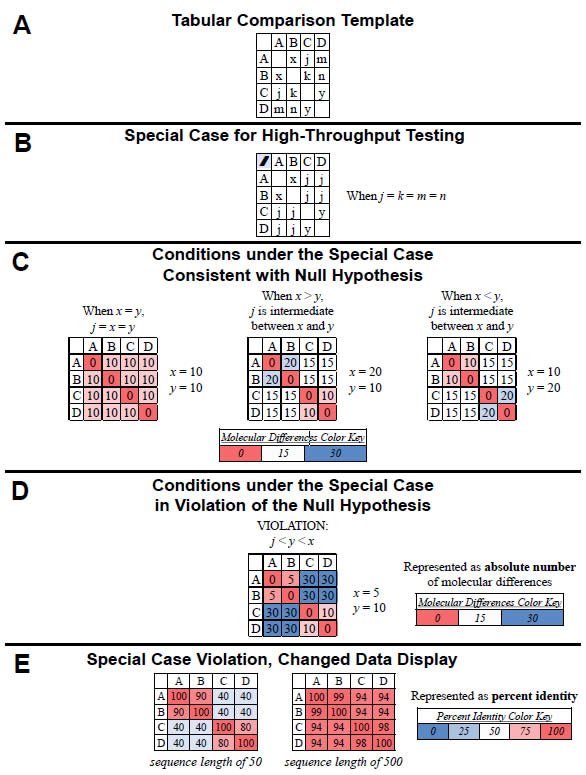
Fig. 1. Testing the null hypothesis. The null hypothesis can be tested in a high-throughput manner using a tabular heat-mapped display. (A) For four “kinds” (A, B, C, D), the comparisons between individual pairs of “kinds” are represented by x (A–B comparison), j (A–C comparison), m (A–D comparison), k (B–C comparison), n (B–D comparison), and y (C–D comparison). (B) When the four inter-group comparisons (A–C, A–D, B–C, B–D) yield equivalent values (i.e., j = k = m = n), the number of variables reduces to three (x, y, j). (C) When the four intergroup comparisons (A–C, A–D, B–C, B–D) yield equivalent values (i.e., j = k = m= , as per [B]), three cases exist for which the null hypothesis is valid: When the value of j is equivalent to the values of x and y (see left-hand table) and when the value of j is intermediate between x and y (two cases of this: When x > y and when x < y or; see center and right-hand tables). These conditions are readily visible when the values are heat-mapped by color (see color key). (D) When the four intergroup comparisons (A–C, A–D, B–C, B–D) yield equivalent values [i.e., j = k = m = n, as per the conditions in (B)], the null hypothesis is invalid if neither of the conditions in (C) is satisfied—for example, if j is less than both y and x. This violation of the null is easily recognizable visually when the values are heat-mapped by color (see color key). (E) The same data as (D), but converted to percent identity based on a sequence length of either 50 (left-hand table) or 500 (right-hand table). Again, the violation of the null is recognizable visually when the values are heat-mapped by color (see color key).
Heat-mapping these results (see color key in Fig. 1C) permits rapid visual identification of the cases for which the null hypothesis is valid (Fig. 1C). Specifically, as long as the colors of the four intergroup comparisons (i.e., the four j values) either match the colors of original comparisons (see left-most table in Fig. 1C) or are intermediate in color between the color of the original comparisons (see center and right-most tables in Fig. 1C), then the null hypothesis is valid.
Conversely, using example values for x, y, and j, violations of the null hypothesis can be visualized easily. For example, if x = 5 and y = 10, the null hypothesis is true only if the value of j is intermediate in value between x and y (i.e., if j = 7.5). [Proof: x + y = 2j; 5 + 10 = 2j; 15 = 2j; 7.5 = j]. If the value of j is not intermediate in value (e.g., j = 30), then the null is violated (Fig. 1D).
Heat-mapping this result permits rapid identification of this case as a violation of the null (Fig. 1D). In general, when the colors of the four intergroup comparisons neither match the colors of original comparisons (x and y) and nor are intermediate in color between the colors of the original comparisons (x and y), then the null hypothesis is violated, as per the example in Fig, 1D.
Percent Identity Displays
I used a slightly modified version of this heat-mapped display due to several practical limitations of my mitochondrial DNA analysis methods. First, my choice of sequence alignment algorithm limited the types of sequences I could compare. All multiple-sequence alignment algorithms assume a model of sequence change (Morrison 2006), and each algorithm is sensitive to only a subset of types of molecular differences. The algorithm I used, CLUSTALX (Larkin et al. 2007; Thompson, Higgins and Gibson 1994), assumes a simple model of sequence change and, therefore, performs well on alignments of sequences with point mutations or small insertions/deletions, but performs poorly on alignments of sequences with significant structural rearrangements (i.e., translocations). Since mitochondrial gene order differs dramatically among metazoan species (Supplemental Table 1), I limited my kingdom-wide comparisons with CLUSTALX to individual protein sequences instead of whole mitochondrial genome sequences.
Second, differences in protein sequence length across all ~2700 metazoan species (see Supplemental Tables 2–14) limited the manner in which I reported the results of my comparisons. Given these length differences, it is difficult to measure absolute molecular differences among different species. In contrast, reporting differences as percent identity for those positions that actually aligned (i.e., not for positions which represent gaps or overhangs) compensates for these differences in length. Since all change is random under the null hypothesis, this “snapshot” method for reporting results models whole protein changes, though it ultimately underestimates total mutational events since it ignores insertions and deletions. Thus, I reported all my molecular differences in terms of percent identity, not in terms of absolute levels of molecular change.
Visualizing Results as Percent Identity
Visualizing pairwise “kind” comparisons as percent identity values rather than absolute molecular difference values still permits rapid identification of violations of the null hypothesis. For example, using the same data from Fig. 1D and converting the values to percent identity (assuming a sequence length of 50), the heat-mapped results identified a violation of the null hypothesis just as well as the heat-mapped absolute difference results (compare left-hand table in Fig. 1E to Fig. 1D). In both tables, the colors of the four inter-group comparisons (i.e., the value of j) neither matched the colors of original comparisons (x and y) nor were intermediate in color between the colors of the original comparisons (x and y).
Visual identification of violations of the null hypothesis becomes more challenging when molecular differences represent a small fraction of the total sequence length, but it is still feasible. For example, if I assumed a sequence length of 500 for the comparisons in Fig. 1D, converting the differences to percent identity led to a display where the colors seemed to blend together. However, violation of the null was still apparent upon close inspection since the colors of the four intergroup comparisons (i.e., the value of j) neither matched the colors of original comparisons (x and y) nor were intermediate in color between the colors of the original comparisons (x and y). When sequences from curated databases are used, identifying small differences is realistic. When non-curated sequences are used, this sort of analysis becomes unreliable.
This high-throughput visual display of percent identities is useful for recognizing violations of the null even when j is not precisely equivalent to k, m, and n. As long as these four variables are roughly equivalent, and as long as each of these variables individually is much less in value than either x or y, it is easy to recognize violations. In this latter case, the four variables (j, k, m, n) will share a color much different than x or y, and the condition which violates the null (j < both x and y) will be readily apparent.
Summary
- Significant technological hurdles prevent the interrogation of the origin and function of molecular diversity across a large number of animal “kinds” from a young-earth creation perspective using traditional methods.
- As an alternative approach, I derived a method in which a strict null hypothesis is created to be refuted, and the refutation identifies (by process of elimination) the true explanation for the function of molecular differences.
- Directional change is the signature result by which the null hypothesis can be refuted.
- Directional change can be identified when groups of “kinds” are compared to one another but not when members of the same “kind” are compared to one another since members of the same “kind” can produce directional change via hybridization.
- Special mathematical cases exist which allow rapid, high-throughput testing and refutation of the null hypothesis.
- Under these special cases, use of percent identity displays and of heat-mapping allows rapid visual identification of violations of the null hypothesis.
Explaining Molecular Diversity Within “Kinds”
Could the metazoan mitochondrial DNA and protein datasets also be used to test hypotheses for the molecular differences within “kinds”? In principle, yes. In practice, the answer to this question becomes more challenging.
Several methods do not lend themselves to testing hypotheses for differences within “kinds.” Refutation of the null hypothesis cannot be used as a method since it applies only to comparisons of individuals belonging to separate “kinds.” Members of the same “kind” may have shared ancestries due to breeding, and this fact violates the foundational requirement of testing the null hypothesis, namely, separate ancestries among the individuals compared. Systematic mutagenesis also cannot be used since testing all of the intra-“kind” differences is cost and time prohibitive. Hence, at present, population modeling is the only feasible means which to test hypotheses on within-“kind” molecular differences.
The chief intra-“kind” hypotheses to be tested are whether individual members of the same “kind” were created with identical sequences or with different sequences during the Creation week, and whether modern differences represent functional or neutral changes since creation. The hypothesis of created diversity cannot be tested for “kinds” that later boarded the Ark two-by-two (e.g., felids [Pendragon and Winkler 2011]) since the bottleneck of the Flood effectively narrowed the mitochondrial DNA population to a single sequence, assuming that the female that boarded the Ark did not possess heteroplasmic mitochondrial DNA sequences. For “kinds” that survived outside the Ark (e.g., fish), the effects of the Flood on “kind” populations sizes is unknown, and population modeling may reveal which hypothesis is true.
The existence of fossil DNA sequences does not aid in answering these questions. DNA is a labile molecule, and it is difficult to imagine that DNA could survive without degradation for thousands of years, as Criswell (2009) has already discussed. Though some signatures of DNA degradation are known, it seems impossible to know all the signatures of DNA degradation until some independent means of evaluating fossil DNA sequences is discovered. Until then, the reliability of fossil DNA sequences will remain a perpetual mystery, and fossil DNA cannot be used to inform hypotheses on within-‘kind’ molecular differences.
Despite these historical and practical constraints, it is still a valuable exercise to test whether modern sequence diversity can be traced back to an original starting sequence. For “kinds” that boarded the Ark and, therefore, had a single starting sequence by definition, performing this calculation may reveal new insights into aspects of the post-Flood diversification process, such as the timing of diversification and the constancy of the mutation rate. Performing this exercise for off-Ark “kinds” might test the plausibility of the two chief hypotheses above—whether individual members of off-Ark “kinds” were created with identical sequences or with sequence diversity.
Attempting to trace diversity back to a single starting sequence is, in essence, a coalescence calculation. Because I focused my studies on mitochondrial sequences rather than nuclear sequences, I eliminated the complicating elements of sexual reproduction, diploid states, and recombination from the coalescence equation. Mitochondrial genomes are thought to be uniparentally inherited and to not recombine, making population models simpler. Hence, the equation for mitochondrial DNA coalescence is as follows (after Futuyma 2009, p. 273):
- Let d represent base pair differences between two individuals
- Let r represent the mutation rate
- Let tCA represent time to a common ancestor
- The relationship among these variables:
tCA = d/r
With respect to the mutation rate in equation (23), I made two assumptions to make the model more realistic and to make the math simpler. First, I used only empirically determined mutation rates. Unlike most evolutionary molecular “clock” discussions, I did not use the evolutionary time of origin for a species to calculate and calibrate the mutation rate, a practice which is clearly useless to exploring aspects of the young-earth model.
Second, I assumed a constant mutation rate through time. Though recent geologic studies suggest that the earth may have undergone a period of accelerated radioactive decay during the Flood (Vardiman, Snelling, and Chaffin 2005), it is unclear to what extent this phenomenon would have affected the mutation rate in each “kind.”
A recent human population modeling study of mitochondrial DNA differences suggested that the human mutation rate was indeed accelerated in the past (Wood 2012). However, this study failed to convert the previously published human mutation rate for the hyper-variable region (Parsons et al. 1997) to a whole mitochondrial genome rate. When converted to a whole genome rate (assuming an average genome size of 16,568 nucleotides), it is equivalent to 1 substitution per 1.2 generations, not Wood’s statement of “1 substitution in 33 generations” (Wood 2012, p. 23). This new rate differs from the results of Wood’s analysis (~10 substitutions per generation) by a factor of only ~10 instead of his claimed factor of ~333. Furthermore, the entirety of Wood’s conclusions depends on the assumption that DNA sequences obtained from fossils are accurate—a tentative assumption at best, as discussed above. Thus, if mutation rates were accelerated in the past, studies to date have not unequivocally demonstrated this.
The interrogation of molecular differences within a single “kind” requires one additional modification to equation (23). Since mitochondrial DNA is inherited largely uniparentally, differences between separate lineages within a “kind” are erased when two individuals hybridize. If differences still exist between modern individuals within the same “kind,” these differences must represent the accumulation of changes in separate lineages. Hence, the final d will be the sum of (r * tCA) in lineage #1 and of (r * tCA) in lineage #2. Taking into account this fact, and re-arranging equation (23), the new equation for modeling sequence diversity becomes a divergence calculation rather than a coalescence calculation (after Howell et al. 2003):
- d = 2(r * tCA)
Several practical limitations restricted the application of equation (24) across metazoans. First, mitochondrial mutation rates among metazoans have been measured for only four species: Caenorhabditis elegans (Denver et al. 2000), Drosophila melanogaster (Haag-Liautard et al. 2008), Daphnia pulex (Xu et al. 2012), and Homo sapiens (Parsons et al. 1997).
Second, the human mitochondrial mutation rate has been the subject of significant controversy. The early results of Parsons et al. (1997) were met with skepticism from the evolutionary community since the conclusions contradicted the evolutionary timescale (Gibbons 1998). At least 14 additional studies have been published among 13 individual reports, with strongly disputed conclusions (Bendall et al. 1996; Cavelier et al. 2000; Heyer et al. 2001; Howell, Kubacka, and Mackey 1996; Howell et al. 2003; Janzin et al. 1998; Madrigal et al. 2012; Mumm et al. 1997; Parsons and Holland 1998; Santos et al. 2005; Santos et al. 2008; Sigurðardóttir et al. 2000; Soodyall et al. 1997).
Finally, species representation in the RefSeq database is low for the families to which C. elegans, D. melanogaster, and D. pulex belong. Though many species are known to exist within these families, mitochondrial genome sequences have been determined for very few of these species. Since the taxonomic rank of family seems to approximate the “kind” ancestry boundary (Wood 2006b), this meant that within-“kind” molecular diversity was poorly represented in the RefSeq database for the three “kinds.”
In this study, I addressed each of these problems separately. Though only four species possess measured mutation rates, these four species represent three distinct phyla, which together represent a significant fraction of all animal life. Hence, conclusions obtained from these four species have implications for large swaths of life.
However, the “kinds” to which the three animal species belong possess numerous other species. It is unknown whether all the species within a single “kind” mutate at the same rate. For simplicity, I assumed that all the species within a “kind” changed at the same rate.
With respect to the specific controversy over the human mutation rate, I recalculated a pooled rate from these experiments after taking into account the statistical power in each report (see Materials and Methods section).
The lack of full sequence representation for each “kind” is a significant limitation of this study. Any conclusions based on the sequence diversity known at present may change with the publication of additional sequences from other members of each “kind.” Though this limitation is somewhat compensated by the assumption of a uniform mutation rate for all members of the “kind,” the results of the population modeling in this study are preliminary.
Thus, I attempted to trace modern sequence diversity back to a single starting sequence within each of the Homo, Drosophila, Caenorhabditis, and Daphnia genera using equation (24). The latter three genera represent “kinds” that were likely not on the Ark. Hence, a match between the predictions from equation (24) and modern genetic diversity within these genera (or species) would lend support to the hypothesis that God created the individual members of each “kind” with identical mitochondrial DNA sequences.
I also used equation (24) to test the plausibility of the timescales of the creation and evolution models. Because equation (24) contains a time factor, it implicitly tests the time component of any population genetic model examined. Furthermore, little has been published from a molecular perspective which compares the creation and evolution models on the question of the age of the earth. Comparing evolutionary predictions based on empirically derived mutation rates to modern genetic diversity might be revealing. Conflicts between the two could lead to a new argument against the millions-of-years timescale.
Summary
- Rejection of the null hypothesis does not apply to comparisons within the same “kind” since individual members of the same “kind” can hybridize.
- Population modeling addresses the identity of the original starting sequence within “kinds,” but mutation rates are known for only four species.
- Population modeling within “kinds” is also a test of the young-earth and evolutionary timescales.
Materials and Methods
Sequence retrieval
Whole mitochondrial genome sequence entries from 2704 species/entries were downloaded from the NCBI Nucleotide Reference Sequence (RefSeq) database (http://www.ncbi.nlm.nih.gov/nucleotide/) on July 18, 2012. A Python script was written and used to extract the relevant NCBI identification information, taxonomic ranking labels, and protein or whole genome sequences from the GenBank file, and the extracted information was used to populate a Microsoft Access database (see Supplemental Tables 15 and 16 for NCBI identification numbers for each sequence). Missing information (due to limitations of the Python algorithm) was manually entered into the database either from the NCBI website or the original GenBank flat file. Queries were run on the Access database to obtain relevant information (i.e., protein sequence, classification, genome size, etc.). Sequence files were sorted alphabetically based on classification rank and label, and then saved in CLUSTALX-compatible format.
Gene Order Retrieval
The gene order of the mitochondrial protein-coding genes for select metazoan species was downloaded from the NCBI Organellar Genome Resources website (http://www.ncbi.nlm.nih.gov/genomes/GenomesHome.cgi?taxid=2759&hopt=html) on July 18, 2012, and imported into a Microsoft Excel file for manual color-coding and analysis. A single species was assigned to each row. Each row contained (in left-to-right order) the (1) NCBI accession number for the whole genome sequence for the species, (2) the manually color-coded protein-coding gene order for the species, and (3) the taxonomic rank and label information for the species (which was used to sort the species vertically). Gene abbreviations were as follows: ATP synthase subunit 6 (“ATP6”), ATP synthase subunit 8 (“ATP8”), cytochrome c oxidase subunits 1–3 (“COX1”, “COX2”, “COX3”), cytochrome B (“CYTB”), and NADH dehydrogenase subunits 1-6 (“ND1”, “ND2”, “ND3”, “ND4”, “ND4L”, “ND5”, “ND6”).
Protein sequence analysis
Protein sequences (ordered by species based on alphabetically sorted taxonomic rank and label) from each species were aligned with CLUSTALX (2.1) software (http://www.clustal.org/clustal2/) and run in multiple alignment mode using default parameters, with the exception of changing the output order to “input” (to preserve the taxonomically ranked order of the sequences). Sequences from each of the 13 mitochondrial proteins were aligned separately. For example, all species possessing an ATP synthase subunit 6 (“ATP6”) protein sequence were aligned together, and all species possessing an ATP synthase subunit 8 (“ATP8”) protein sequence were aligned together. In each alignment, ~2600–2700 metazoan species were represented.
Alignment files were imported into a Microsoft Excel spreadsheet with a single, large heat-mapped table assigned to the results of each of the 13 mitochondrial protein sequence alignments. Amino acids in each table were color-coded. One species was assigned to each row. Each row contained (in left-to-right order) the (1) taxonomic rank and label information for each species, which was used to sort the species vertically (larger taxonomic groups were manually color-coded for easier visualization), and (2) the CLUSTALX-aligned and manually color-coded amino acid sequence for the species.
Percent identity matrices were created from the results of each individual alignment and imported into a Microsoft Excel spreadsheet. A single species was assigned to a single row and to a single column. The vertical order of species along the y axis (top to bottom) was identical to the horizontal order of species along the x axis (left to right). Taxonomic information for each species was placed in the same row as each species. Larger taxonomic groups were manually color-coded for easier visualization. Percent identity values were heat-mapped using Excel conditional formatting with a sliding color scale (dark blue = 0%, white = 50%, bright red = 100%). Hence, the percent identity for a comparison of two species’ sequences was found at the intersection of the row (column) for the first species and the column (row) for the second species. The entirety of the heat map in an individual table was captured by zooming out from the individual data points, and these images were displayed in Figs. 2–14 in this paper.
Protein statistics were calculated from the database created above and from alignment results. The average protein size for a given protein was calculated from the length of each species’ amino acid sequence entry in the RefSeq database. The average percent identity for a given protein was calculated from the table of percent identity results above after first removing all the “100%” values that represented comparisons of a species to itself (which would automatically yield a value of 100% identity). The results for both of these statistical analyses were heat-mapped using Microsoft Excel conditional formatting with a sliding color scale (dark blue = lowest value, white = 50th percentile, bright red = highest value).
Taxonomy template creation
Each species possessing an ATP synthase subunit 6 (“ATP6”) protein sequence was compared in tabular format based on the species’ taxonomic rank and label for the four higher-level Linnaean taxonomic categories (kingdom, phylum, class, order [no intermediate categories between them]), as per the NCBI labels assigned to each species. The only exceptions I made to the NCBI labels were as follows: I placed Crocodylidae, Testudines, Sphenodontia, and Squamata into a single class, Reptilia (they were separated taxonomically in the NCBI database). I labeled Ruminatia as an order (it was listed it as a sub-order in the NCBI database), and I labeled Suina and Tylopoda as orders (the NCBI database did not).
Table 1. Summary of published human mitochondrial DNA mutation rate studies.
Published studies (D-loop region)
| Paper | Method of Detection | Number of Detected Mutants | Generations (transmissions) | Base Pairs (bp) | bp * Generations | Ethnicity |
|---|---|---|---|---|---|---|
| Bendall 1996 | Heteroplasmy | 4 | 360 | 313 | 112680 | |
| Cavelier 2000 | Homoplasmy | 0 | 292 | 792 | 231264 | Swedish |
| Heyer 2001 | Homoplasmy | 4 | 508 | 673 | 341884 | French-Quebecois |
| Howell 1996 | Heteroplasmy | 2 | 88 | 1194 | 105072 | Australian |
| Howell 2003 | Heteroplasmy | 1 | 185 | 1122 | 207570 | European |
| Howell 2003 (UTMB) | Heteroplasmy | 3 | 263 | 1122 | 295086 | |
| Janzin 1998 | Homoplasmy | 0 | 228 | 370 | 84360 | Swedish |
| Madrigal 2012 | Homoplasmy | 2 | 220 | 360 | 79200 | Costa Rica |
| Mumm 1997 | Homo/heteroplasmy | 1 | 59 | 443 | 26137 | |
| Parsons 1997 | Homo/heteroplasmy | 10 | 327 | 610 | 199470 | European origin |
| Parsons 1998 | Heteroplasmy | 10 | 306 | 610 | 186660 | |
| Santos 2005 | Heteroplasmy | 6 | 321 | 973 | 312333 | Azores Islands |
| Sigurðardóttir 2000 | Homo/heteroplasmy | 5 | 705 | 673 | 474465 | Icelanders |
| Soodyall 1997 | Homoplasmy | 0 | 108 | 698 | 75384 | Tristan da Cunha |
Published Studies (Coding Region)
| Paper | Method of Detection | Number of Detected Mutants | Generations (transmissions) | Base Pairs (bp) | BP * Generations | Ethnicity |
| Cavelier 2000 | Homoplasmy | 0 | 256 | 365 | 93440 | Swedish |
| Howell 2003 | Heteroplasmy | 4 | 170 | 15447 | 2625990 | European |
| Santos 2008 | Heteroplasmy | 2 | 311 | 1102 | 342722 | Azores Islands |
Table 2. Statistical power for human coding region study.
| Modern pairwise difference (average for non-Africans) | Average size of coding region | Approximate generations since Adam | Required mutation rate for 6000 origin of modern sequences (mutants/bp/generation) | Paper | Measured bp* generations | Expected mutants in 6000 years |
| 29.9 | 15,447 | 200 | 4.84E-06 | Cavelier 2000 | 93,440 | 0.5 |
Species were arrayed by assigning each species to a single row and to a single column. The vertical order of species along the y axis (top to bottom) was identical to the horizontal order of species along the x axis (left to right). Taxonomic information for each species was placed in the same row as each species.
Differences in classification rank and label between two species were used to manually create a table where 1 = the two belong to different phyla; 2 = same phylum, different classes; 3 = same class, different order; and 4 = same order. All values were heat-mapped using Microsoft Excel conditional formatting with a sliding color scale (dark blue = 1, white = 2.5, bright red = 4). The entirety of the heat map was captured by zooming out from the individual data points, and this image was displayed in Fig. 15.
Genetic Diversity Predictions
Empirically determined mitochondrial mutation rates (“mutations/generation”) for C. elegans, D. melanogaster, and D. pulex were obtained from the literature (Denver et al. 2000; Haag-Liautard et al. 2008; Xu et al. 2012). Mitochondrial mutation rates (“mutations/ generation”) for H. sapiens were also obtained from the literature (Bendall et al. 1996; Cavelier et al. 2000; Heyer et al. 2001; Howell et al. 1996; Howell et al. 2003; Janzin et al. 1998; Madrigal et al. 2012; Mumm et al. 1997; Parsons et al. 1997; Parsons and Holland 1998; Santos et al. 2005; Santos et al. 2008; Sigurðardóttir et al. 2000; Soodyall et al. 1997).
A pooled human mitochondrial mutation rate was calculated from the published base substitution rates in the literature (Bendall et al. 1996; Cavelier et al. 2000; Heyer et al. 2001; Howell et al. 1996; Howell et al. 2003; Janzin et al. 1998; Madrigal et al. 2012; Mumm et al. 1997; Parsons et al. 1997; Parsons and Holland 1998; Santos et al. 2005; Santos et al. 2008; Sigurðardóttir et al. 2000; Soodyall et al. 1997). These published studies conflict on the rate of mitochondrial DNA change, reflected in the number of mutants reported for each study (Table 1). They also differ in statistical power (e.g., base pairs measured, transmission events), in the ethnic group surveyed, in the type of mutation measured (homoplasmic versus heteroplasmic), and in the region of the mitochondrial genome surveyed (e.g., D-loop or coding region) (Table 1).
Only those studies which measured the mutation rate from homoplasmic changes were included for further analysis since the fate of heteroplasmic mutations is unknown. This effectively narrowed the available results for the D-loop region to seven studies since the Mumm et al. (1997) study did not give sufficient data to determine the rate of homoplasmic changes (Table 1).
This also effectively eliminated all coding region results. Strictly homoplasmic studies on the coding region of the mitochondrial genome exist for only a single study (Table 1). However, this study had poor statistical power. Given the average number of modern pair-wise nucleotide differences among non- Africans (Kim and Schuster 2013), the average size of the coding region of the mitochondrial genome, and the approximate number of generations since Adam, the average mutation rate required to explain modern diversity on a young-earth timescale can be calculated (Table 2). This rate predicts that Cavelier et al. (2000) would have found less than one mutation in their study, given the number of total base pairs (bp * generations) they examined (Table 2). Hence, this study was excluded from further consideration, effectively limiting the present analysis to the D-loop region of the human mitochondrial genome.
Comparing the remaining seven D-loop region studies that reported homoplasmic mutations revealed a striking trend between statistical power and number of mutations detected (Table 3). The three studies with the highest number of detected mutations had the highest level of statistical power, as measured either by number of pedigrees analyzed or by a product of the number of base pairs surveyed and the generations examined (Table 3). Conversely, one of the studies with the lowest number of detected mutations (zero) (Soodyall et al. 1997) also had the lowest level of statistical power as measured by total pedigrees surveyed (Table 3). Of the remaining two studies which reported zero mutations (Cavelier et al. 2000; Janzin et al. 1998), the latter also had low statistical power, as measured by a product of the number of base pairs surveyed and the generations examined (Table 3). Together, these trends suggested that the “contradictions” among these studies may simply be an artifact of the statistical power of each study.
In light of these facts, I recalculated a mutation rate for the human D-loop region factoring in the statistical power inherent to each published study. I pooled the raw data for number of mutants detected, and I pooled the results of the product of the number of generations surveyed and number of base pairs analyzed. This effectively weighs each study by the total number of base pairs analyzed. I used these pooled values to calculate an average mutation rate in terms of mutants per base pair per generation (Table 4).
Table 4. Average mutation rate for the human D-loop region (homoplasmy studies only).
| Paper | Homoplasmic substitutions | Generations (transmissions) | base pairs (BP) | bp * generations | Ethnicity | Average mutants/ (bp * generation) |
| Cavelier 2000 | 0 | 292 | 792 | 231,264 | Swedish | 1.08E-05 |
| Heyer 2001 | 4 | 508 | 673 | 341,884 | French-Quebecois | |
| Janzin 1998 | 0 | 228 | 370 | 84,360 | Swedish | |
| Madrigal 2012 | 2 | 220 | 360 | 79,200 | Costa Rica | |
| Parsons 1997 | 7 | 327 | 610 | 199,470 | European origin | |
| Sigurðardóttir 2000 | 3 | 705 | 673 | 474,465 | Icelanders | |
| Soodyall 1997 | 0 | 108 | 698 | 75,384 | Tristan da Cunha | |
| Total | 16 | 1,486,027 |
This rate was used to predict divergence in the D-loop region among modern humans (Supplemental Table 17). First, the mutation rate was converted to “mutations/year/D-loop region” using a range of generation time estimates and the published length of the D-loop region (Kim and Schuster 2013). Second, predicted divergence was calculated by multiplying the mutation rate for a given generation time by two and by the time of origin (as per equation [24]). Time of origin for the creation model was assumed to be a rounded upper-limit date for the Creation week, 10,000 years ago. The time of origin for the evolutionary model was determined from the literature (Soares et al. 2009). Ninety-five percent confidence intervals were calculated by treating the discovery of mutants in the D-loop as a Poisson-distributed event. The 95% confidence interval (CI) for Poisson data can be calculated as follows (Supplemental Table 17):
- Let λ represent the average mutation rate
- Let ν represent the sample size (in this case, number of pooled generational events)
- CI = λ ± 1.96[√(λ/ν)]
The predictions were compared to the published mitochondrial D-loop diversity for Homo sapiens (Kim and Schuster 2013). Ideally, my predictions should have been compared to the results of a different study since my pooled mutation rate was derived from non-African ethnic groups and since the data from Kim and Schuster included African sequences (Table 4). However, the African sequences in the Kim and Schuster study represented less than 10% of the total sequences, and since their results represented over 7,000 individuals, I used their data without further modification.

Fig. 2. Kingdom-wide violations of the null hypothesis with ATP6 alignments.
Proteins sequences for ATP synthase subunit 6 (“ATP6”) were compared across metazoan species, and the percent identity values for each species-species comparison were heat-mapped (see color key at right). Since individual species were not discernible at this level of zooming, major taxonomic groups of species were highlighted with orange bars along the horizontal and vertical axes. As visible in this display, clusters of high identity were evident, and they corresponded to groups of species sharing a taxonomic rank above the level of family, some of which have been identified explicitly (e.g., the class Mammalia, near the lower center-right of the table). Furthermore, when these groups (clusters) of species were compared against one another, violations of the null hypothesis were immediately observable, as per the criteria depicted on the right—clusters of high identity (representing x and y) were dissimilar from one another (the junction between the clusters represents j). Individual data points can be viewed in Supplemental Table 22.
Similar predictions were made for Caenorhabditis, Drosophila, and Daphnia (Supplemental Table 18). Published base substitution rates were converted to “mutations/year/genome” with the average of the RefSeq-listed genome size for each genus and with the generation time estimates for C. elegans, D. melanogaster, and D. pulex from the literature (Denver et al. 2000; Xu et al. 2012) and from academic websites (http://genome.wustl.edu/genomes/view/caenorhabditis_elegans/, accessed September 6, 2012; http://flystocks.bio.indiana.edu/Fly_Work/culturing.htm, accessed September 6, 2012).
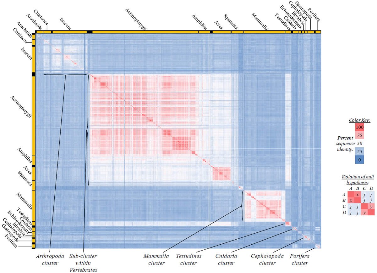
Fig. 3. Kingdom-wide violations of the null hypothesis with ATP8 alignments.
Proteins sequences for ATP synthase subunit 8 (“ATP8”) were compared across metazoan species, and the percent identity values for each species-species comparison were heat-mapped (see color key at right). Since individual species were not discernible at this level of zooming, major taxonomic groups of species were highlighted with orange bars along the horizontal and vertical axes. As visible in this display, clusters of high identity were evident, and they corresponded to groups of species sharing a taxonomic rank above the level of family, some of which have been identified explicitly (e.g., the class Mammalia, near the lower center-right of the table). Furthermore, when these groups (clusters) of species were compared against one another, violations of the null hypothesis were immediately observable, as per the criteria depicted on the right—clusters of high identity (representing x and y) were dissimilar from one another (the junction between the clusters represents j). Individual data points can be viewed in Supplemental Table 23.
Since mutation rates for two different lines of D. melanogaster were reported, the average of the two was used in this study. Also, the mutation rates for sexually reproducing D. pulex and asexually reproducing D. pulex were reported, and the average of these two was used in this study.
The 95% confidence intervals for these converted mutation rates were calculated separately for each bound of the interval. The upper bound was calculated by multiplying the upper value of the published 95% confidence interval for the mutation rate by the average genome size, and then by dividing by the shortest generation time (in years) for the species. The lower bound was calculated by multiplying the lower bound of the published 95% confidence interval for the mutation rate by the average genome size, and then by dividing by the longest generation time (in years) for the species (Supplemental Table 18). For Drosophila, the upper and lower bounds were not averaged from the two lines; rather, the highest and lowest reported bounds were used. For Daphnia, the 95% confidence intervals were calculated using only the range of generation times since a 95% confidence interval was not published for the mutation rate (Xu et al. 2012).
Fig. 4. Kingdom-wide violations of the null hypothesis with COX1 alignments.
Proteins sequences for cytochrome c oxidase subunit 1 (“COX1”) were compared across metazoan species, and the percent identity values for each species-species comparison were heat-mapped (see color key at right). Since individual species were not discernible at this level of zooming, major taxonomic groups of species were highlighted with orange bars along the horizontal and vertical axes. As visible in this display, clusters of high identity were evident, and they corresponded to groups of species sharing a taxonomic rank above the level of family, some of which have been identified explicitly (e.g., the class Mammalia, near the lower center-right of the table). Furthermore, when these groups (clusters) of species were compared against one another, violations of the null hypothesis were immediately observable, as per the criteria depicted on the right—clusters of high identity (representing x and y) were dissimilar from one another (the junction between the clusters represents j). Individual data points can be viewed in Supplemental table 24.
Predictions of genetic diversity in these invertebrates were calculated for the creation and evolution models by multiplying the converted mutation rate above by two and by the time of origin (as per equation [24]) (Supplemental Table 19). Time of origin for the creation model was assumed to be a rounded upper-limit date for the Creation week, 10,000 years ago. The time of origin for the evolutionary model was determined from the literature for each genus or species (Cutter 2008; Haag et al. 2009; Obbard et al. 2012).
These predictions were compared to the average genetic diversity within each genus. For the Caenorhabditis, Drosophila, and Daphnia, average diversity was calculated by performing whole genome alignments with CLUSTALX (2.1) software. Drosophila and Caenorhabditis whole genome sequences were downloaded from the RefSeq database as specified above, and all Daphnia whole genome sequences from RefSeq and non-RefSeq NCBI databases were downloaded on March 26, 2013. All “Ns” were removed from Daphnia sequences before aligning them to one another.
All six Drosophila RefSeq entries (melanogaster, mauritiana, sechellia, simulans, yakuba, littoralis) were aligned to one another, and all Daphnia isolates were aligned to one another. Both Caenorhabditis RefSeq entries (elegans, briggsae) were aligned to one another. However, since the gene order data (Supplemental Table 1) indicated that C. elegans and C. briggsae possessed the same genes but in a reverse complementary order, the C. briggsae genome sequence was converted to its reverse complement (http://www.bioinformatics.org/sms/rev_comp.html) before aligning the sequences from the two species.
Fig. 5. Kingdom-wide violations of the null hypothesis with COX2 alignments.
Proteins sequences for cytochrome c oxidase subunit 2 (“COX2”) were compared across metazoan species, and the percent identity values for each species-species comparison were heat-mapped (see color key at right). Since individual species were not discernible at this level of zooming, major taxonomic groups of species were highlighted with orange bars along the horizontal and vertical axes. As visible in this display, clusters of high identity were evident, and they corresponded to groups of species sharing a taxonomic rank above the level of family, some of which have been identified explicitly (e.g., the class Mammalia, near the lower center-right of the table). Furthermore, when these groups (clusters) of species were compared against one another, violations of the null hypothesis were immediately observable, as per the criteria depicted on the right—clusters of high identity (representing x and y) were dissimilar from one another (the junction between the clusters represents j). Individual data points can be viewed in Supplemental Table 25.
Absolute nucleotide differences were calculated for each alignment (Supplemental Table 20). Percent identity matrices were created for the Drosophila and Caenorhabditis alignments and used to calculate average absolute nucleotide differences in two steps. First, the average percent difference was calculated by subtracting the average percent identity from 100. Second, the average absolute difference was calculated by dividing the average percent difference by 100 and then multiplying it by the average genome size for the genus. Also, for the Drosophila alignments, the range of maximum and minimum absolute nucleotide differences was calculated using the maximum and minimum interspecies percent identity values. At the multiplication step of this calculation, the smallest genome size of the two species compared was used since the CLUSTALX alignment algorithm reports percent identity values only for the positions that actually aligned.
The maximum pair-wise difference (rather than the average pair-wise difference) was determined for the D. pulex isolates after correcting for differences in sequence length between the isolates compared. It was calculated by first subtracting the minimum percent identity from 100, and then dividing this number by 100 and multiplying it by the appropriate genome size of the isolates compared. Maximum difference was determined in order to represent the maximum amount of genetic divergence that could have occurred since the D. pulex isolates split off from one another.
As a practical measure of the relationship between the origins model timescale and modern genetic diversity, “years until a single mutation” were calculated (Supplemental Table 21). First, the required average mutation rates for the biblical and evolutionary timescales were calculated by dividing the average genetic diversity for the genus or species by the model-specific timescale. Second, this value and the published mutation rate values were inverted (1/value) to calculate how many years would elapse before a single mutation was observed.
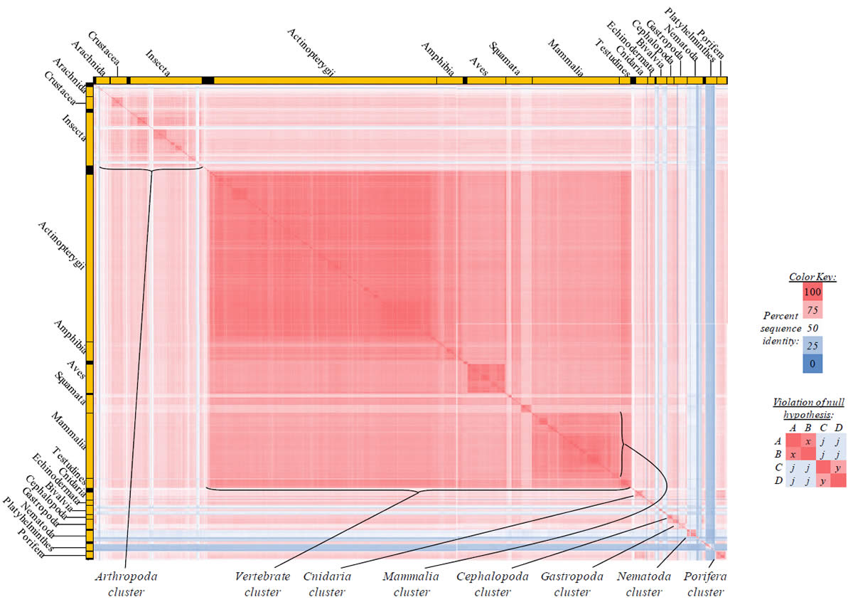
Fig. 6. Kingdom-wide violations of the null hypothesis with COX3 alignments.
Proteins sequences for cytochrome c oxidase subunit 3 (“COX3”) were compared across metazoan species, and the percent identity values for each species-species comparison were heat-mapped (see color key at right). Since individual species were not discernible at this level of zooming, major taxonomic groups of species were highlighted with orange bars along the horizontal and vertical axes. As visible in this display, clusters of high identity were evident, and they corresponded to groups of species sharing a taxonomic rank above the level of family, some of which have been identified explicitly (e.g., the class Mammalia, near the lower center-right of the table). Furthermore, when these groups (clusters) of species were compared against one another, violations of the null hypothesis were immediately observable, as per the criteria depicted on the right—clusters of high identity (representing x and y) were dissimilar from one another (the junction between the clusters represents j). Individual data points can be viewed in Supplemental Table 26.
Results
Kingdom-wide violations of the null hypothesis among different “kinds”
The alignment of each of the 13 mitochondrial protein sequences across thousands of metazoan species revealed three major patterns (Figs. 2–14). First, large groups of species naturally formed visually identifiable groups of high identity (i.e., the red and white “boxes” in Figs. 2–14; see percent identity color key at the right of each figure). For example, a cluster of species of high molecular identity was consistently recognizable in the upper left-hand corner of each table in all mitochondrial proteins examined (white- to red-colored “box” or cluster in Figs. 2–14). Conversely, one to three clusters of species were consistently identifiable in the center of the table in all mitochondrial proteins aligned (white- to red-colored “boxes” or clusters in Figs. 2–14). Several other smaller clusters were consistently visible in the lower right-hand corner of each table as well (Figs. 2–14; see also Supplemental Tables 22–34 for individual data points).
Second, these clusters of high molecular identity corresponded, largely, to classification categories above the taxonomic rank of family. For example, the cluster in the upper left-hand corner of each table corresponded to the phylum Arthropoda (including the class Arachnida, the subphylum Crustacea, and the class Insecta) (Figs. 2–14—compare the red- to white-colored box to the color-coded bars along the horizontal and vertical axes). Conversely, the single large cluster in the center of most tables contained a large subset of the vertebrate species [including the classes Actinopterygii, Aves, Amphibia, and Mammalia, and members (Squamata, Testudines) of the former class Reptilia] (Figs. 2–14—compare red and white-shaded box to the color-coded bars along the horizontal and vertical axes). Also, smaller clusters in the lower right-hand corners of most tables identified the rest of the major phyla, including Cnidaria, Echinodermata, Mollusca (including the classes Bivalvia, Cephalopoda, Gastropoda), Nematoda, Platyhelminthes, and Porifera (Figs. 2–14—compare the red- and white-shaded boxes in the lower right-hand corner to the color-coded bars along the horizontal and vertical axes; see also Supplemental Tables 22–34 for individual data points and details on taxonomic rankings and labels).
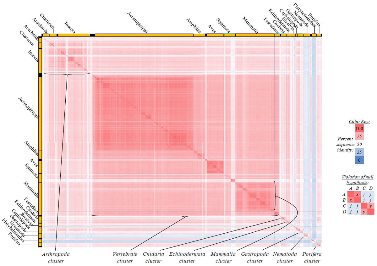
Fig. 7. Kingdom-wide violations of the null hypothesis with CYTB alignments.
Proteins sequences for cytochrome b (“CYTB”) were compared across metazoan species, and the percent identity values for each species-species comparison were heat-mapped (see color key at right). Since individual species were not discernible at this level of zooming, major taxonomic groups of species were highlighted with orange bars along the horizontal and vertical axes. As visible in this display, clusters of high identity were evident, and they corresponded to groups of species sharing a taxonomic rank above the level of family, some of which have been identified explicitly (e.g., the class Mammalia, near the lower center-right of the table). Furthermore, when these groups (clusters) of species were compared against one another, violations of the null hypothesis were immediately observable, as per the criteria depicted on the right—clusters of high identity (representing x and y) were dissimilar from one another (the junction between the clusters represents j). Individual data points can be viewed in Supplemental Table 27.
These results were not limited to the taxonomic rank of phylum. For example, a cluster of high identity near the center of the table and within the vertebrate cluster was consistently identifiable across each mitochondrial protein analyzed (Figs. 2–14), and it corresponded to the class Aves (compare red- and white-shaded box to the taxonomically labeled bars along the horizontal and vertical axes in Figs. 2–14). Also, a cluster of high identity near the lower right-hand side of the table was found across all proteins examined, and it corresponded to the class Mammalia (compare red- and white-shaded box to the taxonomically labeled bars along the horizontal and vertical axes in Figs. 2–14; see also Supplemental Tables 22–34 for individual data points).
Practically, these observations meant that clusters identified “kinds” or groups of “kinds.” Since previous studies found that the taxonomic rank of family approximated the ancestry limit for each “kind” (Wood 2006b), these large clusters of high identity in Figs. 2–14 allowed the rapid visual identification of “kinds” and of clusters of several “kinds,” a necessary condition for testing the null hypothesis.
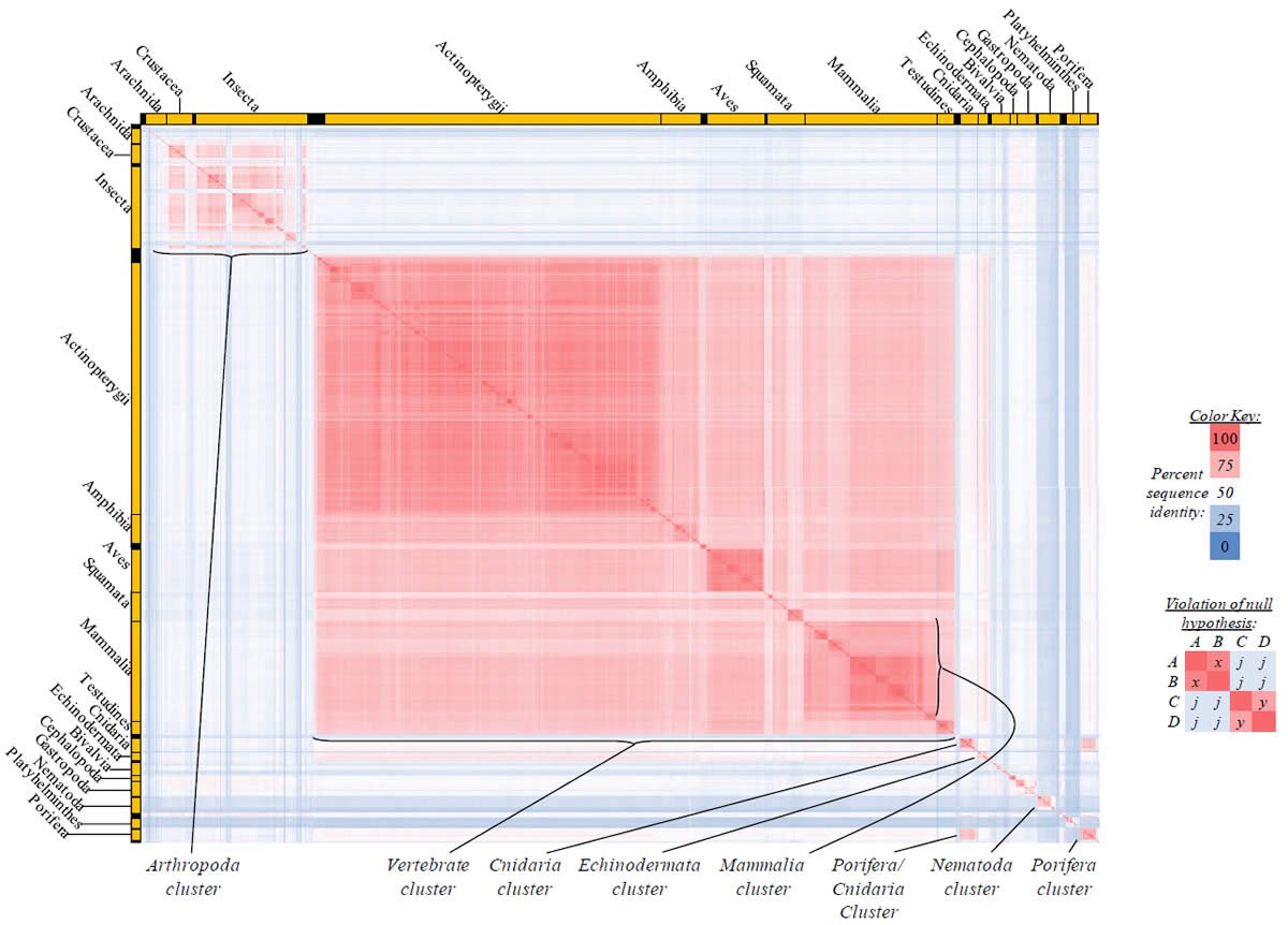
Fig. 8. Kingdom-wide violations of the null hypothesis with ND1 alignments.
Proteins sequences for NADH dehydrogenase subunit 1 (“ND1”) were compared across metazoan species, and the percent identity values for each species-species comparison were heat-mapped (see color key at right). Since individual species were not discernible at this level of zooming, major taxonomic groups of species were highlighted with orange bars along the horizontal and vertical axes. As visible in this display, clusters of high identity were evident, and they corresponded to groups of species sharing a taxonomic rank above the level of family, some of which have been identified explicitly (e.g., the class Mammalia, near the lower center-right of the table). Furthermore, when these groups (clusters) of species were compared against one another, violations of the null hypothesis were immediately observable, as per the criteria depicted on the right—clusters of high identity (representing x and y) were dissimilar from one another (the junction between the clusters represents j). Individual data points can be viewed in Supplemental Table 28.
Third, the percent identity between any two of these large clusters of high identity was low. For example, in Fig. 2, the color of the intersection between the Arthropoda (phylum) cluster and the Mammalia (class) clusters was blue (taxonomically labeled bars along the horizontal and vertical axes identify the intersection between Arthropoda and Mammalia on the upper and/or left side of the table; see also Supplemental Table 22 for individual data points)—representing much lower percent identity than either the arthropod species compared to one another (upper left-hand corner, white to red in color), or the mammalian species compared to one another (lower right-hand side of table, red in color). This relative hierarchy of percent identity among the comparisons between and within the Arthropoda and Mammalia clusters was consistent across each mitochondrial protein analyzed, though the absolute values for each cluster varied (i.e., the colors shifted), depending on the protein analyzed (Figs. 2–14), but not on the average size of the protein analyzed (Table 5).
Conversely, in Fig. 2, the intersection between the subcluster within vertebrates (including the classes Actinopterygii, Amphibia, and Aves, and parts of the order Squamata) and the cluster of nematodes (phylum Nematoda) was dark blue (taxonomically labeled bars along the horizontal and vertical axes identify the intersection between these clusters at the bottom and/or right side of the table; see also Supplemental Table 22 for individual data points)—representing much lower percent identity than either the vertebrate species compared to one another (red in color), or the nematode species compared to one another (red in color) (see also Supplemental Table 22 for individual data points). This relative hierarchy of percent identity among the comparisons between and within these two groups was consistent across each mitochondrial protein analyzed, though the absolute values for each cluster varied (i.e., the colors shifted), depending on the protein analyzed (Figs. 2–14), but not on the average size of the protein analyzed (Table 5).
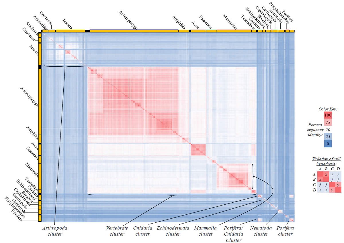
Fig. 9. Kingdom-wide violations of the null hypothesis with ND2 alignments.
Proteins sequences for NADH dehydrogenase subunit 2 (“ND2”) were compared across metazoan species, and the percent identity values for each species-species comparison were heat-mapped (see color key at right). Since individual species were not discernible at this level of zooming, major taxonomic groups of species were highlighted with orange bars along the horizontal and vertical axes. As visible in this display, clusters of high identity were evident, and they corresponded to groups of species sharing a taxonomic rank above the level of family, some of which have been identified explicitly (e.g., the class Mammalia, near the lower center-right of the table). Furthermore, when these groups (clusters) of species were compared against one another, violations of the null hypothesis were immediately observable, as per the criteria depicted on the right—clusters of high identity (representing x and y) were dissimilar from one another (the junction between the clusters represents j). Individual data points can be viewed in Supplemental Table 29.
In summary, numerous visually identifiable clusters of high identity across the entire animal kingdom matched this relative hierarchical pattern—high identity within each cluster, low identity between two clusters. Whether the cluster corresponded to phylum Arthropoda or the phylum Cnidaria, or even to the class Mammalia, a cluster of high identity could be compared to another cluster of high identity, and the identity between these two clusters was lower than the identity within each cluster (Figs. 2–14; see also Supplemental Tables 22–34).
Together, these observations broadly refuted the null hypothesis as the explanation for the origin of these sequences in each of these “kinds” and groups of “kinds.” Refutation of the null hypothesis under the special case (where j = k= m= n, or where j is roughly equivalent k, m, and n) required that j be less than both x and y (see example table on the right-hand side of Figs. 2–14). In each of these tables, x and y were readily identifiable as entire clusters of data points of high identity (Figs. 2–14; see also Supplemental Tables 22–34 for individual data points), representing “kinds” or groups of “kinds.” Conversely, the intersection between each cluster of high identity represented the j, k, m, and n variables. The values of these latter four variables were roughly equivalent to one another, and they were consistently less than both x and y. Since the value of j need not be a specific absolute value (i.e., it need not be colored blue or white, but could even be light red in color), these violations of the null (j < both x and y) refuted the null hypothesis as an explanation for the origin of these proteins among “kinds.”
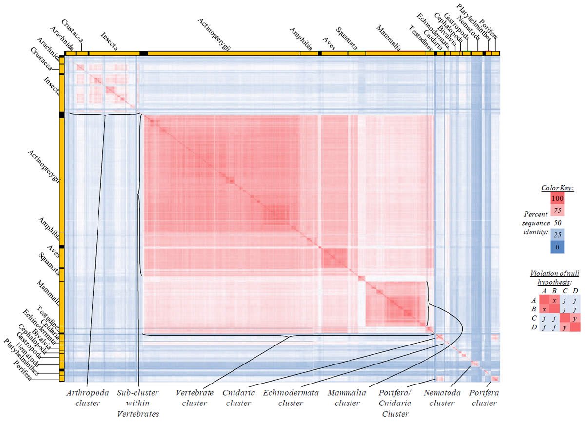
Fig. 10. Kingdom-wide violations of the null hypothesis with ND3 alignments.
Proteins sequences for NADH dehydrogenase subunit 3 (“ND3”) were compared across metazoan species, and the percent identity values for each species-species comparison were heat-mapped (see color key at right). Since individual species were not discernible at this level of zooming, major taxonomic groups of species were highlighted with orange bars along the horizontal and vertical axes. As visible in this display, clusters of high identity were evident, and they corresponded to groups of species sharing a taxonomic rank above the level of family, some of which have been identified explicitly (e.g., the class Mammalia, near the lower center-right of the table). Furthermore, when these groups (clusters) of species were compared against one another, violations of the null hypothesis were immediately observable, as per the criteria depicted on the right—clusters of high identity (representing x and y) were dissimilar from one another (the junction between the clusters represents j). Individual data points can be viewed in Supplemental Table 30.
Additionally, these results implied that, not only mitochondrial proteins, but also the entire mitochondrial genome sequence in each “kind” could not be explained by the null hypothesis. Since the DNA coding for these 13 proteins together comprised most of the mitochondrial genome sequence in most species (data not shown), the null was violated for a large fraction of the total genome sequence. Conversely, since the entire mitochondrial genome (not subsections which code for individual protein sequences) is passed on largely uniparentally and without recombining from generation to generation (Al Rawi et al. 2011; Sato and Sato 2011), violation of the null hypothesis for part of the genome sequence meant violation of the null for the whole genome sequence.
Identification of mitochondrial protein function
These results also implied that the modern mitochondrial sequence differences among “kinds” represented functional differences. Since the two tenets of the null hypothesis were (1) identical starting sequence and (2) random change, one or both of these tenets must have been wrong, and the alternatives to each of these tenets implied function. If tenet (1) was wrong, meaning that God created sequences different in one or “kinds,” this fact would have implied function for these sequences, since God does not create haphazardly or accidentally. (Again, for the present study I assumed away the hypothesis that certain genetic sequences were created solely for artistic purposes, a hypothesis seemingly in conflict with recent studies [ENCODE Project Consortium 2012]).
Alternatively, if tenet (2) was wrong, non-random change would have also implied function for modern sequence differences. For example, if natural selection were the mechanism, selection would have required a molecular function upon which to act. Conversely, if non-random mutation were the mechanism, this would have implied purpose and function due to the non-random nature of the process (e.g., the rag genes, which fulfill a very specific purpose in the immune system). Thus, modern mitochondrial sequence differences between the “kinds” investigated in this study represented functional differences, not “leftovers” of a neutral change process.
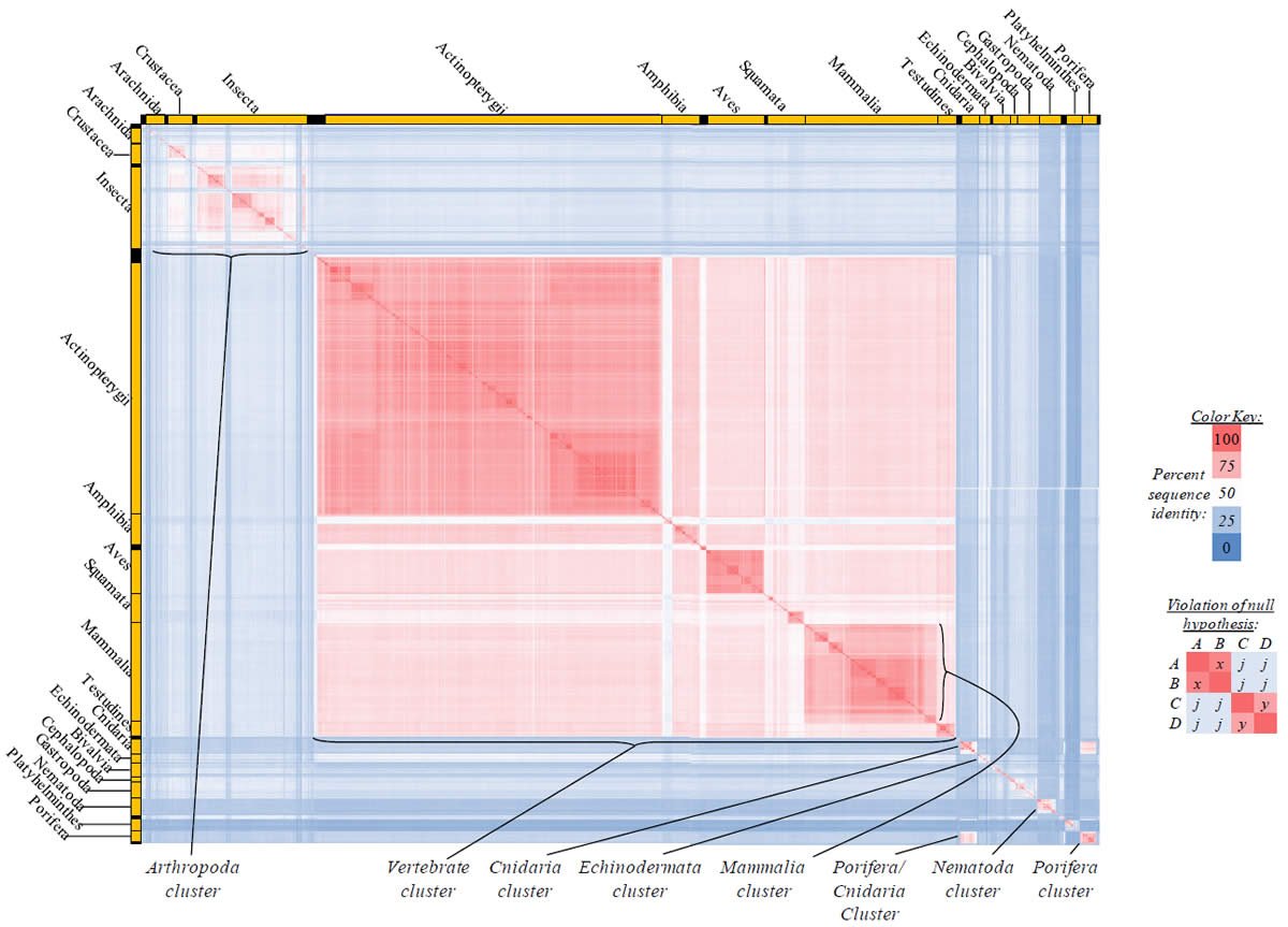
Fig. 11. Kingdom-wide violations of the null hypothesis with ND4 alignments.
Proteins sequences for NADH dehydrogenase subunit 4 (“ND4”) were compared across metazoan species, and the percent identity values for each species-species comparison were heat-mapped (see color key at right). Since individual species were not discernible at this level of zooming, major taxonomic groups of species were highlighted with orange bars along the horizontal and vertical axes. As visible in this display, clusters of high identity were evident, and they corresponded to groups of species sharing a taxonomic rank above the level of family, some of which have been identified explicitly (e.g., the class Mammalia, near the lower center-right of the table). Furthermore, when these groups (clusters) of species were compared against one another, violations of the null hypothesis were immediately observable, as per the criteria depicted on the right—clusters of high identity (representing x and y) were dissimilar from one another (the junction between the clusters represents j). Individual data points can be viewed in Supplemental Table 31.
What function might these individual differences perform? Several functional hypotheses could be invoked to explain the clustering patterns observed in the mitochondrial protein sequences. However, since the clusters of high percent identity seemed to correlate with taxonomic rank above the level of family (Figs. 2–14), I explored whether taxonomic rank would precisely predict the clusters that formed. If taxonomic rank did precisely identify the clusters which naturally formed, this result would imply a taxon-specific function for these amino acid differences.
Toward this end, I created a predictive, heat-mapped template based on the four higher-level Linnaean taxonomic categories [kingdom, phylum, class, order (no intermediate categories between them)] (Fig. 15). I based my template on the species with an ATP synthase subunit 6 (“ATP6”) entry, since the number of species (2697) with an ATP6 protein was close to the total number downloaded species/entries, 2704.
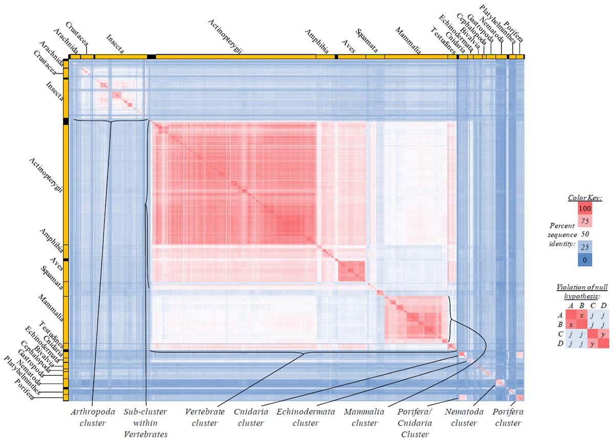
Fig. 12. Kingdom-wide violations of the null hypothesis with ND4L alignments.
Proteins sequences for NADH dehydrogenase subunit 4L (“ND4L”) were compared across metazoan species, and the percent identity values for each species-species comparison were heat-mapped (see color key at right). Since individual species were not discernible at this level of zooming, major taxonomic groups of species were highlighted with orange bars along the horizontal and vertical axes. As visible in this display, clusters of high identity were evident, and they corresponded to groups of species sharing a taxonomic rank above the level of family, some of which have been identified explicitly (e.g., the class Mammalia, near the lower center-right of the table). Furthermore, when these groups (clusters) of species were compared against one another, violations of the null hypothesis were immediately observable, as per the criteria depicted on the right—clusters of high identity (representing x and y) were dissimilar from one another (the junction between the clusters represents j). Individual data points can be viewed in Supplemental Table 32.
This artificial taxonomic template (Fig. 15) clearly identified some of the clustering patterns I observed for the mitochondrial protein sequence alignments (R2 value between Fig. 2 and Fig. 15 is equal to 0.79). For example, the template identified the Arthropoda and vertebrate clusters, as well as the Actinopterygii, Aves, Mammalia, and Testudines clusters (compare Fig. 15 to Figs. 2–14). The template also isolated some of the major phyla, such as Cnidaria, Echinodermata, Nematoda, and Porifera (Fig. 15). However, the template did not identify all the clusters observable in the protein alignment results, such as the sub-cluster within vertebrates (including the classes Actinopterygii, Aves, Amphibia, and Mammalia, and members [Squamata, Testudines] of the former class Reptilia). It also failed to identify the clustering that occurred among Cnidaria and Porifera (compare Fig. 2 to Fig. 15). Thus, the overlap between the taxon-based heat map and protein sequence-based heat map indicated that taxonomic rank and grouping partially explained the clusters but did not explain all the mitochondrial protein sequence patterns.
Together, these results suggested that amino acid differences between “kinds” function in part in traits unique to each taxon.
Recent origin of mitochondrial genomes
What might be the explanation for molecular differences within “kinds”? Equation (24) was used to predict within-“kind” mitochondrial genetic diversity on both the evolutionary and young-earth timescales.
Comparison of the predictions of the evolutionary model and of the young-earth model to actual diversity within the Caenorhabditis, Drosophila, Daphnia, and Homo genera (see Supplemental Tables 22–34 for calculations) strongly refuted the evolutionary model but supported the young-earth model of a constant mutation rate and single starting sequence within each genus or species. The 95% confidence intervals for the predictions of the creation model captured or overlapped actual genetic diversity for three of the four genera (Fig. 16A–B, D), and the predictions for the remaining genus (Daphnia) were still within an order of magnitude of the modern value (Fig. 16C) (see also Supplementary Tables 19–20).
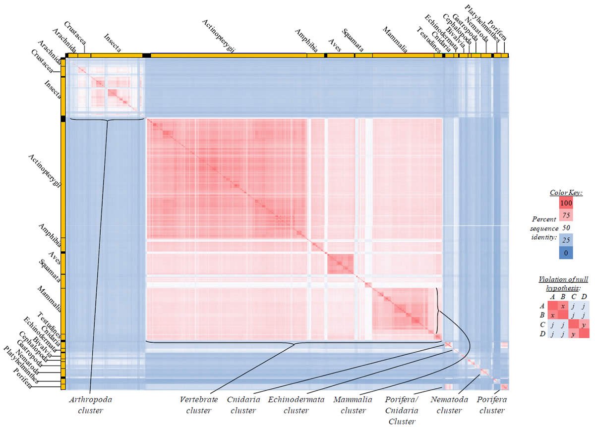
Fig. 13. Kingdom-wide violations of the null hypothesis with ND5 alignments.
Proteins sequences for NADH dehydrogenase subunit 5 (“ND5”) were compared across metazoan species, and the percent identity values for each species-species comparison were heat-mapped (see color key at right). Since individual species were not discernible at this level of zooming, major taxonomic groups of species were highlighted with orange bars along the horizontal and vertical axes. As visible in this display, clusters of high identity were evident, and they corresponded to groups of species sharing a taxonomic rank above the level of family, some of which have been identified explicitly (e.g., the class Mammalia, near the lower center-right of the table). Furthermore, when these groups (clusters) of species were compared against one another, violations of the null hypothesis were immediately observable, as per the criteria depicted on the right—clusters of high identity (representing x and y) were dissimilar from one another (the junction between the clusters represents j). Individual data points can be viewed in Supplemental Table 33.
In contrast, the evolutionary model made diversity predictions that were orders of magnitude different from both the young-earth predictions and the actual diversity within each genus (Fig. 16A–D). (Note that though the errors for the evolutionary predictions may appear large, they do not represent the standard deviation but, rather, the 95% confidence intervals. As such, they depict the maximum possible range of predictions for the evolutionary model.) Clearly, the young-earth model came close to the real value while the evolutionary model could not predict reality.
The evolutionary model could not be rescued by assuming a slower rate of change in the past. The minimal mutation rate required to explain modern genetic diversity on an evolutionary timescale was orders of magnitude different from the modern rate of change (Table 6; see also Supplemental Table 21 for calculations). The required rate was so slow that it defied plausibility; a rate of 1 mutation per genome per 20,000–36,000 years—and consistently so for millions of years—implied DNA polymerase and DNA repair fidelity far beyond known levels (Lodish et al. 2000).
Thus, modern genetic diversity argued strongly against the evolutionary timescale and for the young-earth timescale. Though the young-earth population model I used to predict genetic diversity made over-simplifying assumptions, it represented a first approximation, and, as such, it still argued strongly against the evolutionary timescale and suggested that within-“kind” and within-human mitochondrial DNA diversity was largely explicable in terms of a constant mutation rate over 6000–10,000 years of time from a genus-specific starting sequence.
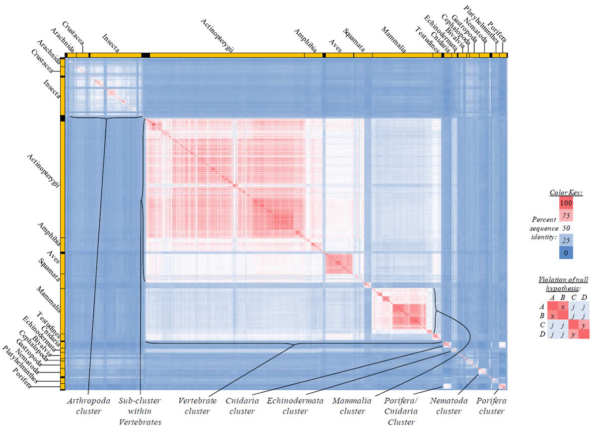
Fig. 14. Kingdom-wide violations of the null hypothesis with ND6 alignments.
Proteins sequences for NADH dehydrogenase subunit 6 (“ND6”) were compared across metazoan species, and the percent identity values for each species-species comparison were heat-mapped (see color key at right). Since individual species were not discernible at this level of zooming, major taxonomic groups of species were highlighted with orange bars along the horizontal and vertical axes. As visible in this display, clusters of high identity were evident, and they corresponded to groups of species sharing a taxonomic rank above the level of family, some of which have been identified explicitly (e.g., the class Mammalia, near the lower center-right of the table). Furthermore, when these groups (clusters) of species were compared against one another, violations of the null hypothesis were immediately observable, as per the criteria depicted on the right—clusters of high identity (representing x and y) were dissimilar from one another (the junction between the clusters represents j). Individual data points can be viewed in Supplemental Table 34.
Together, these population modeling conclusions and the results from testing of the null hypothesis in a kingdom-wide manner suggested that molecular patterns within “kinds” were due to constant mutation over time from a genus-specific starting sequence, and that molecular patterns between “kinds” were explicable in functional terms.
Discussion
A predictive young-earth model
Table 5. Overall statistics for taxa-wide protein comparisons.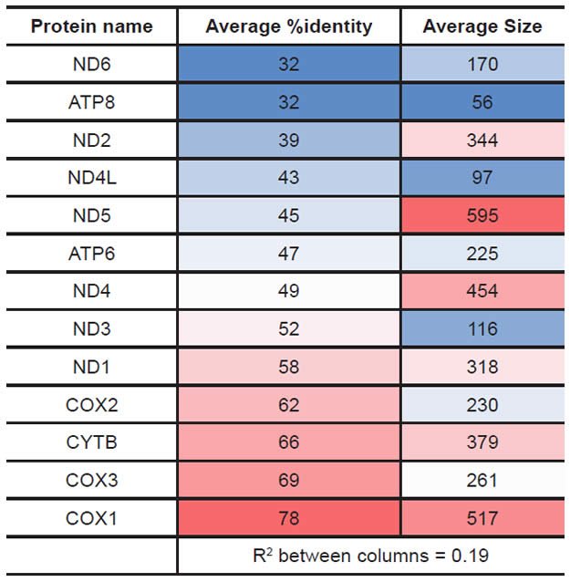
What is the explanation for molecular diversity? The derivation of equation (7) and the successful use of equation (24) add predictive rigor to the young-earth model of molecular differences. Instead of vague generalities, these equations offer testable, quantitative estimates of protein function and genetic diversity across the entire animal kingdom. No longer are these molecular parameters exclusively a function of “evolutionary conservation” or of time since evolutionary divergence. Rather, equations (7) and (24) provide compelling alternative methods based on the young-earth timescale and the biblical limits on ancestry. This represents a key step forward in developing the creation model.
These new tools could theoretically be applied to a variety of remaining young-earth biology questions. For example, equations (7) and (24) could be used to investigate the origins of mitochondrial DNA differences of plants, fungi, and protists. In addition, equation (7) could be used on comparisons of other molecules besides mitochondrial DNA. The null hypothesis could be tested for other classes of proteins, such a transcription factors, and for other types of sequences, such as non-coding RNA. The full potential for these equations is yet to be realized.
Explaining molecular diversity between “kinds”
Applied to mitochondrial proteins of metazoans, equation (7) demonstrates that the individual amino acid differences between “kinds” are inconsistent with neutral change from a single starting sequence. This failure of the null hypothesis to account for the origin of modern mitochondrial sequences raises the question of which assumption of the model is in error. The alternatives to random change include non-random mutation and natural selection. However, with respect to the latter, recent research indicates that natural selection is very poor at creating new protein sequences (Behe 2007). Conversely, if non-random mutation were the explanation, several different mutases mutating at gene-specific rates would be needed since the levels of absolute protein sequence diversity vary among the mitochondrial proteins (Table 5). Since very few site-specific mutases are currently known, nonrandom mutation seems even less likely of an explanation than natural selection.
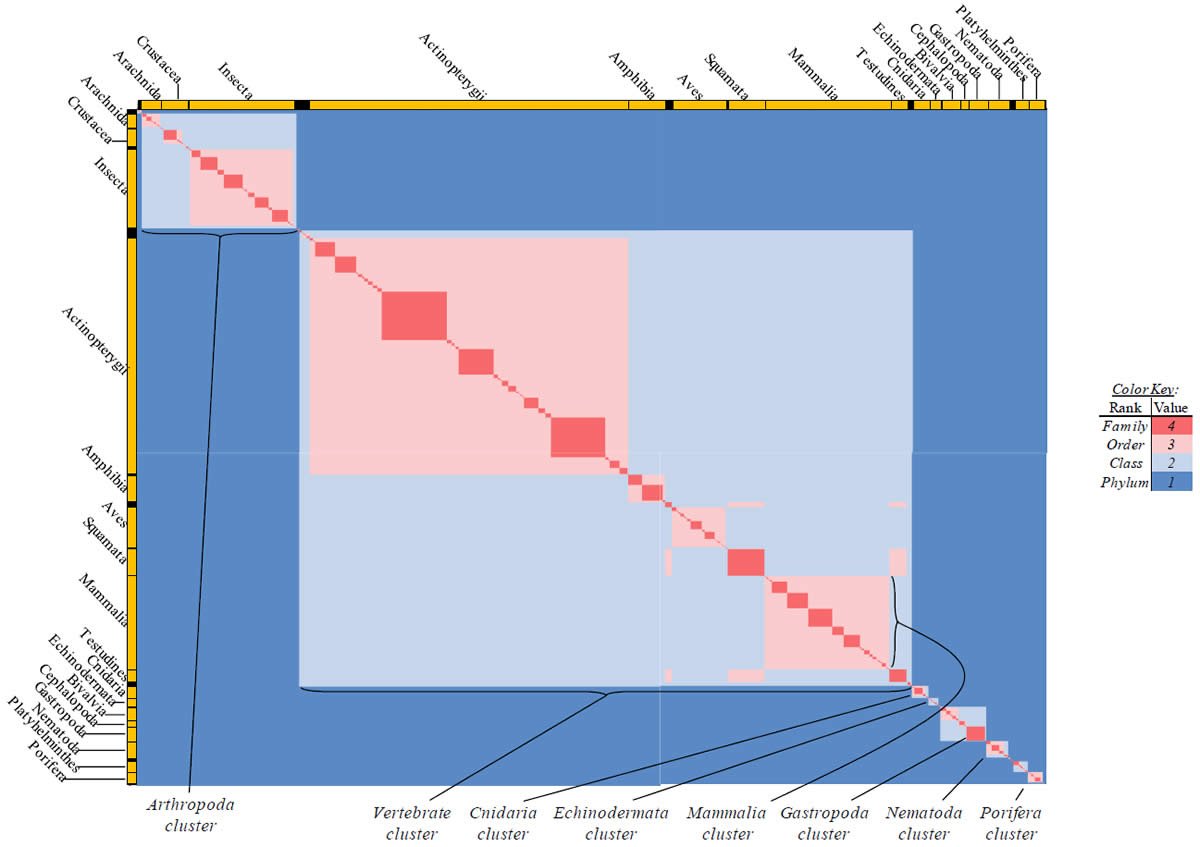
Fig. 15. Predictive taxonomy template produces observable clusters.
Each species possessing an ATP synthase subunit 6 (“ATP6”) protein sequence was compared based on the species’ taxonomic rank and label, and the results of these pair-wise comparisons were heat-mapped (see color key). Since individual species were not discernible at this level of zooming, major taxonomic groups of species were highlighted with orange bars along the horizontal and vertical axes. As visible in this display, clustering patterns were immediately evident, some of which have been identified explicitly (e.g., the class Mammalia, near the lower center-right of the table). These patterns replicated some, but not all, of the clustering patterns observable in Fig. 2 (R2 value between Fig. 2 and Fig. 15 is equal to 0.79). Individual data points can be viewed in Supplemental Table 35.
Nonrandom change might also be explicable by thermodynamic constraints. No amino acid or nucleotide residue exists in isolation, and perhaps the sequences that God created during the Creation week narrow the possible options for change post-Creation. In essence, this explanation is a form of negative selection—that mutations occur randomly with respect to sequence position but that existing functional constraints make the outcome of this process nonrandom. Strict mathematical elimination of this hypothesis is beyond the scope of this study, and a comprehensive elimination of this hypothesis seems difficult since the full functions of DNA and proteins are just beginning to be understood. However, given the size of the mitochondrial genome (~16,500 base pairs for humans) and the magnitude of the differences among protein sequences among metazoans (Figs. 2–14), an enormous amount of mutational “tries” seems to be required for negative selection (thermodynamic constraint) to be the explanation for change over just 6000 years. Hence, the hypothesis of non-random change as a sufficient explanation for the patterns I observed lacks compelling evidence in its favor.
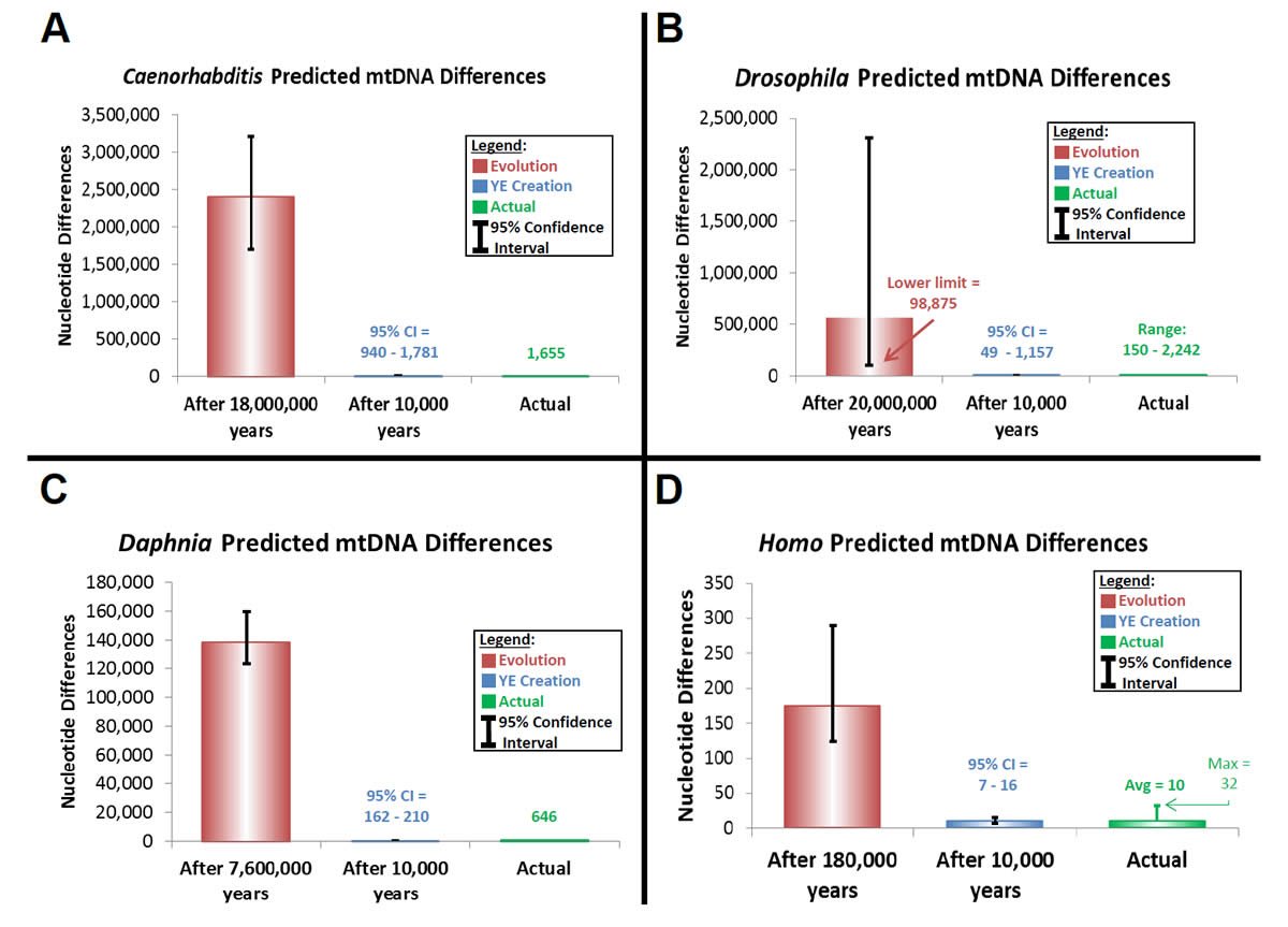
Fig. 16. Recent origin of mitochondrial genome sequences.
Predictions of genetic diversity compared to modern nucleotide diversity within (A) Caenorhabditis species, (B) Drosophila species, (C) Daphnia pulex isolates, and (D) modern Homo sapiens. The height of the bars represents the results of the calculations using the average generation time and average mutation rate. The black bars represent the 95% confidence intervals. See Supplemental Tables 19–20 for calculations.
In contrast, the hypothesis of created diversity is consistent with at least two lines of evidence. First, it is consistent with Scripture and with God’s character that each “kind” would be functionally equipped once, rather than undergo many rounds of successive updates and improvements. Genesis 1 documents God’s global biological creation acts, and other Scriptures (Genesis 2:1–3; Exodus 20:11; Hebrews 4:3) indicate that God’s global creation acts were finished by Day 7. Also, since God is omnipotent and omniscient, we might expect Him to genetically prepare each creature from the start of creation for future challenges, as has already been described in plants for a phenomenon termed “mediated design” (Wood and Cavanaugh 2001, Wood 2003b).
Table 6. Unrealistic mutation rate requirements for the evolutionary timescale
| Years elapsed until a single mutation occurs | |||
|---|---|---|---|
| Genus | Evolution | Creation | Actual |
| Caenorhabditis | 21,752 | 12 | 6–11 |
| Drosophila | 34,247 | 17 | 9–202 |
| Daphnia | 23,259 | 31 | 48–62 |
| Homo | 36,364 | 2,020 | 1,244–2,915 |
Second, the hypothesis of created diversity is consistent with the approximate match between actual genetic diversity and the predictions of the specific young-earth hypothesis tested in this study (Fig. 16). This match suggests that the species within each genus (or individuals within each species) shared the same starting sequence or nearly the same starting sequence. Conversely, since the protein sequences among these four genera are very different (Supplemental Tables 2–14), and since the DNA sequences coding for the compared proteins sequences represent the majority of each mitochondrial genome sequence, the Creation week sequence for each genus was likely unique to each genus. Furthermore, since these population genetic findings are consistent across three independent phyla, these results suggest that “kinds” in general were created with unique sequences.
Thus, the hypothesis that the modern genetic diversity between “kinds” arose by direct act of God during the Creation week is the most plausible explanation at present.
Created diversity likely represents functional diversity. God could have created the sequence differences observed in this study for purely aesthetic reasons, but the strong match between traditional (functional) classification categories and the clusters in this study (Fig. 2 compared to Fig. 15) suggests function for the molecular differences. Thus, the mitochondrial protein differences between “kinds” likely exist for functional reasons.
How do we reconcile this statement with the prevailing view that amino acid residues of “house-keeping” proteins are functionally redundant (McLaughlin Jr. et al. 2012; Theobald 2012)? Overly narrow definitions of terms may be the answer.
A similar type of situation arose in early studies attempting to determine the number of “essential” genes in various organisms. Early genome-wide gene knockout studies in yeast and C. elegans suggested that most genes were not essential (Kamath et al. 2003; Winzeler et al. 1999); however, these studies were performed under a very restricted set of laboratory conditions. More recent studies expanded the set of conditions under which gene function could be tested, and the results of these experiments concluded the opposite—that most genes are essential (Hillenmeyer et al. 2008; Ramani et al. 2012). How were these disparate results reconciled? By carefully defining “essential.” Early studies found that most genes were not “essential”—under standard laboratory conditions. Latter studies found that most genes were “essential”—under at least one type of condition or for a specific level of fitness.
How has “function” for individual amino acid positions been defined under the functional redundancy view (McLaughlin Jr. et al. 2012; Theobald 2012)? Studies to date have been performed in vitro or during restricted windows of embryonic development. Neither of these settings fully explores all the conditions under which amino acids may contribute to function, and many proteins might perform their functions during a period of development that is not currently experimentally accessible. Thus, under the functional redundancy view, “function” has been defined in an overly narrow sense, and the real function of each amino acid position might not be discovered until comprehensive in vivo investigations are performed.
What specific in vivo function might each of these amino acid positions perform? Traditional views of protein function do not typically ascribe roles to individual amino acids (aside from active site residues), but the existence of so many functional clusters of protein diversity (Figs. 2–14) implies many different functions for these protein sequences. Furthermore, the partial match between my taxonomy hypothesis (Fig. 15) and the actual protein sequence clusters (Figs. 2–14) suggests that some of the sequences are involved in traits defining each taxonomic category.
Several hypotheses can be proposed to explain the involvement of mitochondrial proteins with taxon-specific traits. For example, modern protein sequences might still perform the same basal metabolic function traditionally ascribed to them (i.e., participation in the electron transport chain), but the sequence might be optimized metabolically for the specific organismal context in which each protein is found.
Alternatively, each protein might be connected in a genetic network to pathways specifying taxon-specific traits (Lynch, May, and Wagner 2011). The phenomenon of protein “moonlighting” (Jeffery 2003) raises the possibility that the traditional metabolic functions of each mitochondrial protein are just one of many functions for each protein. For example, the electron transport chain protein cytochrome b (“CYTB”) might participate, not just in basal energy transformation, but also in DNA transcription as a transcription factor, similar to the findings for the glycolytic enzyme glyceraldehyde-3-phosphate dehydrogenase (“GAPDH”) (Kim and Dang 2005).
This protein “moonlighting” hypothesis is consistent with the observation that the protein clusters found in this study transcend Linnaean classification categories—categories which sometimes separate (rather than cluster) species that share a functional trait. For example, bony fish, amphibians, birds, and most reptiles share the reproductive strategy of laying eggs, but these species are divided into separate Linnaean classes. In contrast, the ATP6 sequence comparison in this study joined species from Actinopterygii, Amphibia, Aves, and Reptilia into a vertebrate sub-cluster (Fig. 2). Hence, the clustering patterns I observed might be explained in part by functions shared by multiple taxonomic categories.
This potential mechanism of function immediately suggests an answer to a current young-earth research question, the molecular mechanism by which species diversified post-Creation and post-Flood (Parker 1980; Wood 2002; Wood 2003a; Wood 2003b; Wood and Cavanaugh 2001). If each protein sequence was created to participate in many taxon-specific pathways, changing a few amino acids in a single protein may lead to pleiotropic effects. For example, a single mutation in the ATP6 sequence of the Felid “kind” ancestor may have altered not only the efficiency of the electron transport chain in that ancestor but also the ability to produce stripes. Thus, the mechanism of intra-“kind” diversification might be explained in part by a simple molecular process.
Conversely, if proteins were created multi-functional, this would create additional barriers to the step-by-step change that evolution requires. In terms pioneered by the Intelligent Design movement, multi-functionality would represent an additional level of “irreducible complexity” (Behe 1996). For example, if a protein is involved in many genetic networks, this implies that no amino acid position in that protein exists in isolation. Hence, a single amino acid change that produces a positive effect in one pathway may simultaneously interfere with the function of several other pathways, leading to whole system and organismal collapse. This would complicate the steps required to realize large-scale evolutionary change.
Finally, the refutation of the null hypothesis answers the evolutionary challenge of functional redundancy among “house-keeping” protein residues (Theobald 2012). Evolutionists criticize the creation model, wondering why God would create “house-keeping” protein sequences in a manner that strongly suggests common ancestry and evolutionary change through time. Why created “house-keeping” proteins with different sequences when they perform the same function? Apparently, “house-keeping” proteins perform more functions than evolutionists originally concluded, as the results of this study clearly show.
Exhaustive in vivo mutagenesis studies should reveal which model has a better explanation for the molecular patterns between “kinds.” In the meantime, the challenge of “functional redundancy” is premature and, therefore, innocuous.
Explaining molecular diversity within “kinds”
Did God create individual members of a “kind” with the same starting sequences? The results of this study are consistent with this hypothesis. As Fig. 16 demonstrates, modern genetic diversity within a genus or species could be traced back to a single starting sequence for 3 of the 4 groups analyzed, and the fourth group was still within an order of magnitude of the known modern diversity value. This latter discrepancy may be resolved once more Daphnia sequences are curated.
Further refinements to this population model must be made before it can be fully accepted. Species representation is low within the families to which the Caenorhabditis, Drosophila, and Daphnia species belong, and since family seems to be the approximate taxonomic boundary of a “kind” (Wood 2006b), these results do not directly address the question of starting sequences within “kinds.” Also, the results for Homo addressed only the origin of the D-loop, not the entire mitochondrial genome. In addition, the timescale I used represents an upper boundary of the date of the Creation week, not the more likely date of 6000 years. More studies are needed to model these parameters appropriately before the hypothesis of a single starting sequence can be accepted or rejected.
Modeling the young-earth timescale
The results in Fig. 16 provide strong support for the recent origin of mitochondrial genome sequences. The predictions of young-earth timescale fit the actual diversity in all four genera within an order of magnitude (Fig. 16A–D). Though this dataset is limited and, therefore, a first approximation, these data from three independent phyla suggest that modern mutation rates applied over 6000–10,000 years explain mitochondrial diversity within a genus.
These results refute a common old-earth creation objection to the young-earth creation model. Opponents of young-earth creation have criticized the young-earth model for being too much like the evolutionary model in invoking rapid speciation post-Flood (Moore 2004). They view this aspect of young-earth biology as impossible and as a strong argument against the biblical timescale. The results of Fig. 16 answer this challenge. Modern genetic diversity fit the young-earth timescale very well. Not only do these data suggest that rapid change is plausible, they argue that is it real.
Implications for the timescale of evolutionary change
The results of this paper also challenge the evolutionary timescale. The population modeling performed in this study strongly contradicts an ancient (i.e., hundreds of thousands to millions of years) origin for the Caenorhabditis, Drosophila, Daphnia, and Homo genera (Fig. 16A–D). Together, these results from three independent phyla (Nematoda, Arthropoda, and Chordata) present a strong challenge to the evolutionary model for the origin of the species within these phyla.
Might manipulation of population genetic parameters answer this challenge? Calculations of the minimal mutation rate required to explain modern genetic diversity on an evolutionary timescale were so slow that they defied plausibility; a rate of 1 mutation per 20,000–34,000 years (and consistently so for millions of years) implied DNA polymerase and DNA repair fidelity far beyond known levels—perhaps near miraculous (Table 6). Furthermore, evolutionary geologists and astronomers commonly and arbitrarily assume constant rates of change when determining the timescales of history (Lisle 2010; Vardiman, Snelling, and Chaffin 2005). Consistency would demand assuming (arbitrarily) a constant rate of change in biology as well. Thus, slower mutation rates could not reconcile the predictions of the evolutionary model with real diversity.
Coalescence theory also seems to offer little aid to this evolutionary dilemma. If the sequences being compared were nuclear DNA sequences where new alleles can be lost easily due to the facts of biparental inheritance, recombination, and diploidy, perhaps the evolutionary model could invoke genetic drift as an explanation. Instead, these calculations were performed on uniparentally inherited, non-recombining mitochondrial DNA sequences where mutations accumulate over time much faster and have a much greater chance of being fixed in the population. I made the predictions using published methods for coalescence and divergence based on these facts (Futuyma 2009; Howell et al. 2003). The evolutionary model cannot be rescued by random genetic drift.
Finally, natural selection is a poor rescuing device for evolution. If invoked, natural selection is faced with a difficult explanatory task. On one hand, it must explain how, after millions of years of mutation, Caenorhabditis, Drosophila, and Daphnia species have sustained intense genomic mutational change with very little phenotypic consequence (Fig. 16A–C). In the same breath, natural selection must also explain the opposite—how a few mutations in the supposed hominid ancestor of humans and chimpanzees produced enormous phenotypic differences observable between these two species today. This seemingly ad hoc explanation strains credulity.
The only potential rescuing device for evolution is the limits of species’ representation of this study. Perhaps mutation rates will be measured in other species that are dramatically slower than the published rates. Alternatively, perhaps the sequencing of other species within each “kind” will reveal unprecedented levels of genetic diversity more in line with the predictions of millions of years of evolution. Until these data are obtained, the results of this study argue strongly against the evolutionary timescale.
Conclusion
The findings of this study advance the young-earth explanation for molecular diversity. Molecular diversity between “kinds” seems to stem primarily from the creation of diversity during the Creation week. This discovery brings the creation model a step closer to predicting absolute and relative levels of molecular differences between “kinds.” Conversely, molecular diversity within “kinds” appears to be explicable by modern mutation rates applied over the young-earth timescale, with equation (24) adding predictive rigor to this aspect of creation molecular biology. The derivation of equation (7) allows the prediction of molecular function between “kinds,” a key step forward in answering an objection to the young-earth model based on nested hierarchical patterns of sequence diversity between “kinds” (Theobald 2012). Finally, the lack of significant diversity within modern genera and species argues against the ancient (millions of years) origin of modern species. Together, the results of this study significantly advance the young-earth understanding of molecular patterns and present a strong challenge to the timescale of the evolutionary model.
Acknowledgments
Special thanks to Daryl Robbins for Python scripting and database creation. Additional thanks to Paul Nelson and Steve Hopper for stimulating and helpful discussions. Thanks to Jeff Tomkins, Brian Thomas, Frank Sherwin, Robert Carter, Matthew Cserháti, and several other reviewers for helpful comments and criticisms.
References
Al Rawi, S., S. Louvet-Vallée, A. Djeddi, M. Sachse, E. Culetto, C. Hajjar, L. Boyd, R. Legouis, and V. Galy. 2011. Postfertilization autophagy of sperm organelles prevents paternal mitochondrial DNA transmission. Science 334, no. 6059:1144–1147.
Behe, M. J. 1996. Darwin’s black box. New York, New York: Touchstone.
Behe, M. J. 2007. The edge of evolution: The search for the limits of Darwinism. New York, New York: Free Press.
Bendall, K. E., V. A. Macaulay, J. R. Baker, and B. C. Sykes. 1996. Heteroplasmic point mutations in the human mtDNA control region. American Journal of Human Genetics 59, no. 6:1276–1287.
Bergman, J. and J. Tomkins. 2012. Is the human genome nearly identical to chimpanzee?—A reassessment of the literature. Journal of Creation 26, no. 1:54–60.
Carroll, S. B. 2005. Endless forms most beautiful. New York, New York: W. W. Norton & Company.
Cavelier, L., E. Jazin, P. Galonen, and U. Gyllensten. 2000. MtDNA substitution rate and segregation of heteroplasmy in coding and noncoding regions. Human Genetics 107, no. 1:45–50.
Criswell, D. 2009. Neandertal DNA and modern humans. Creation Research Society Quarterly 45, no. 4:246–254.
Cutter, A. D. 2008. Divergence times in Caenorhabditis and Drosophila inferred from direct estimates of the neutral mutation rate. Molecular Biology and Evolution 25, no. 4:778–786.
Dawkins, R. 2009. The greatest show on earth. New York, New York: Free Press.
Denver, D. R., K. Morris, M. Lynch, L. L. Vassilieva, and W. K. Thomas. 2000. High direct estimate of the mutation rate in the mitochondrial genome of Caenorhabditis elegans. Science 289, no. 5488:2342–2344.
Drosophila 12 Genomes Consortium. 2007. Evolution of genes and genomes on the Drosophila phylogeny. Nature 450, no. 7167:203–218.
ENCODE Project Consortium. 2012. An integrated encyclopedia of DNA elements in the human genome. Nature 489, no. 7414:57–74.
Futuyma, D. J. 2009. Evolution. Sunderland, Massachusetts: Sinauer Associates.
Gibbons, A. 1998. Calibrating the mitochondrial clock. Science 279, no. 5347:28–29.
Haag, C. R., S. J. McTaggart, A. Didier, T. J. Little, and D. Charlesworth. 2009. Nucleotide polymorphism and within-gene recombination in Daphnia magna and D. pulex, two cyclical parthenogens. Genetics 182, no. 1:313–323.
Haag-Liautard, C., N. Coffey, D. Houle, M. Lynch, B. Charlesworth, and P. D. Keightley. 2008. Direct estimation of the mitochondrial DNA mutation rate in Drosophila melanogaster. PLoS Biology 6, no. 8:1706–1714.
Heyer, E., E. Zietkiewicz, A. Rochowski, V. Yotova, J. Puymirat, and D. Labuda. 2001. Phylogenetic and familial estimates of mitochondrial substitution rates: Study of control region mutations in deep-rooting pedigrees. American Journal of Human Genetics 69, no. 5:1113–1126.
Hillenmeyer, M. E., E. Fung, J. Wildenhain, S. E. Pierce, S. Hoon, W. Lee, M. Proctor et al. 2008. The chemical genomic portrait of yeast: Uncovering a phenotype for all genes. Science 320, no. 5874:362–365.
Howell, N., I. Kubacka, and D. A. Mackey. 1996. How rapidly does the human mitochondrial genome evolve? American Journal of Human Genetics 59, no. 3:501–509.
Howell, N., C. B. Smejkal, D. A. Mackey, P. F. Chinnery, D. M. Turnbull, and C. Herrnstadt. 2003. The pedigree rate of sequence divergence is the human mitochondrial genome: There is a difference between phylogenetic and pedigree rates. American Journal of Human Genetics 72, no. 3:659–670.
Janzin, E., H. Soodyall, P. Jalonen, E. Lindholm, M. Stoneking, and U. Gyllensten. 1998. Mitochondrial mutation rate revisited: Hot spots and polymorphism. Nature Genetics 18:109–110.
Jeffery, C. J. 2003. Moonlighting proteins: Old proteins learning new tricks. Trends in Genetics 19, no. 8:415–417.
Kamath, R. S., A. G. Fraser, Y. Dong, G. Poulin, R. Durbin, M. Gotta, A. Kanapin, et al. 2003. Systematic functional analysis of the Caenorhabditis elegans genome using RNAi. Nature 421, no. 6920:231–237.
Kim, H. L. and S. C. Schuster. 2013. Poor man’s 1000 genome project: Recent human population expansion confounds the detection of disease alleles in 7,098 complete mitochondrial genomes. Frontiers in Genetics 4:1–13.
Kim, J. and C. V. Dang. 2005. Multifaceted roles of glycolytic enzymes. Trends in Biochemical Sciences 30, no. 3:42–50.
Larkin, M. A., G. Blackshields, N. P. Brown, R. Chenna, P. A. McGettigan, H. McWilliam, F. Valentin, et al. 2007. Clustal W and clustal X version 2.0. Bioinformatics 23, no. 21:2947–2948.
Lisle, J. 2010. Anisotropic Synchrony Convention—A Solution to the Distant Starlight Problem. Answers Research Journal 3:191–207. Retrieved from http://www.answersingenesis.org/articles/arj/v3/n1/anisotropic-synchrony-convention.
Lodish, H., A. Berk, S. L. Zipursky, P. Matsudaira, D. Baltimore, and J. Darnell. 2000. Molecular cell biology. New York, New York: W. H. Freedman and Company.
Lynch, V. J., G. May, and G. P. Wagner. 2011. Regulatory evolution through divergence of a phosphoswitch in the transcription factor CEBPB. Nature 480, no. 7377:383–386.
Madrigal, L., L. Castri, M. Melendez-Obando, R. Villegas-Palma, R. Barrantes, H. Raventos, R. Pereira, D. Luiselli, D. Pettener, and G. Barbujani. 2012. High mitochondrial mutation rates estimated from deep-rooting Costa Rican pedigrees. American Journal of Physical Anthropology 148, no. 3:327–333.
McGee, D. 2012. Creation Date of Adam from the Perspective of Young-Earth Creationism. Answers Research Journal 5:217–230. Retrieved from http://www.answersingenesis.org/articles/arj/v5/n1/age-of-adam.
McLaughlin Jr., R. N., F. J. Poelwijk, A. Raman, W. S. Gosal, and R. Ranganathan. 2012. The spatial architecture of protein function and adaptation. Nature 491, no. 7422:138–142.
Mumm, S., M. P. Whyte, R. V. Thakker, K. H. Buetow, and D. Schlessinger. 1997. mtDNA analysis shows common ancestry in two kindreds with X-linked recessive hypoparathyroidism and reveals a heteroplasmic silent mutation. American Journal of Human Genetics 60, no. 1:153–159.
Moore, G. 2004. Rapid post-flood speciation: A critique of the young-earth model. Retrieved from http://www.reasons.org/articles/rapid-post-flood-speciation-a-critique-of-the-young-earth-model on November 28, 2012.
Morrison, D. A. 2006. Multiple sequence alignment for phylogenetic purposes. Australian Systematic Botany 19:479–539.
Obbard, D.J., J. Maclennan, K.-W. Kim, A. Rambaut, P.M. O’Grady, and F.M. Jiggins. 2012. Estimating divergence dates and substitution rates in the Drosophila phylogeny. Molecular Biology and Evolution 29, no. 11:3459–3473. Retrieved from http://mbe.oxfordjournals.org/content/early/2012/08/10/molbev.mss150.full.pdf+html. on August 29, 2012.
Parker, G. 1980. Creation, mutation, and variation. Acts & Facts. 9, no. 11.
Parsons, T. J. and M. M. Holland. 1998. Mitochondrial mutation rate revisited: Hot spots and polymorphism. Nature Genetics 18:109–110.
Parsons T. J., D. S. Muniec, K. Sullivan, N. Woodyatt, R. Alliston-Greiner, M. R. Wilson, D. L. Berry et al. 1997. A high observed substitution rate in the human mitochondrial DNA control region. Nature Genetics 15, no. 4:363–368.
Pendragon, B. and N. Winkler. 2011. The family of cats—delineation of the feline basic type. Journal of Creation 25, no. 2:118–124.
Ramani, A. K., T. Chuluunbaatar, A. J. Verster, H. Na, V. Vu, N. Pelte, N. Wannissorn, A. Jiao and A. G. Fraser. 2012. The majority of animal genes are required for wild-type fitness. Cell 148, no. 4:792–802.
Santos, C., R. Montiel, A. Arruda, L. Alvarez, M.P. Aluja, and M. Lima. 2008. Mutation patterns of mtDNA: Empirical inferences for the coding region. BMC Evolutionary Biology 8:167.
Santos, C., R. Montiel, B. Sierra, C. Bettencourt, E. Fernandez, L. Alvarez, M. Lima, A. Abade, and M. P. Aluja. 2005. Understanding differences between phylogenetic and pedigree-derived mtDNA mutation rate: A model using families from the Azores Islands (Portugal). Molecular Biology and Evolution 22, no. 6:1490–1505.
Sato, M. and K. Sato. 2011. Degradation of paternal mitochondria by fertilization-triggered autophagy in C. elegans embryos. Science 334, no. 6059:1141–1144.
Sigurðardóttir, S., A. Helgason, J. R. Gulcher, K. Stefansson, and P. Donnelly. 2000. The mutation rate in the human mtDNA control region. American Journal of Human Genetics 66, no. 5:1599–1609.
Soares, P., L. Ermini, N. Thomson, M. Mormina, T. Rito, A. Röhl, A. Salas, S. Oppenheimer, V. Macaulay, and M. B. Richards. 2009. Correcting for purifying selection: An improved human mitochondrial molecular clock. American Journal of Human Genetics 84, no. 6:740–759.
Soodyall, H., T. Jenkins, A. Mukherjee, E. du Toit, D. F. Roberts, and M. Stoneking. 1997. The founding mitochondrial DNA lineages of Tristan da Cunha islanders. American Journal of Physical Anthropology 104, no. 2:157–166.
The Chimpanzee Sequencing and Analysis Consortium. 2005. Initial sequence of the chimpanzee genome and comparison with the human genome. Nature. 437:69–87.
Theobald, D. 2012. 29+ evidences for macroevolution: The scientific case for common descent. Retrieved from http://www.talkorigins.org/faqs/comdesc/ on September 7, 2012.
Thompson, J. D., D. G. Higgins, and T. J. Gibson. 1994. CLUSTAL W: Improving the sensitivity of progressive multiple sequence alignment through sequence weighting, position-specific gap penalties and weight matrix choice. Nucleic Acids Research 22, no. 22:4673–4680.
Tomkins, J. P. 2011. Genome-Wide DNA Alignment Similarity (Identity) for 40,000 Chimpanzee DNA Sequences Queried against the Human Genome is 86–89%. Answers Research Journal 4:233–241. Retrieved from http://www.answersingenesis.org/articles/arj/v4/n1/blastin.
Tomkins, J. P. 2013. Comprehensive Analysis of Chimpanzee and Human Chromosomes Reveals Average DNA Similarity of 70%. Answers Research Journal 6:63–69. Retrieved from http://www.answersingenesis.org/articles/arj/v6/n1/human-chimp-chromosome.
Tomkins, J. and Bergman, J. 2012. Genomic monkey business—estimates of nearly identical human-chimp DNA similarity re-evaluated using omitted data. Journal of Creation 26, no. 1:94–100.
Vardiman, L., A. A. Snelling and E. F. Chaffin, eds. 2005. Radioisotopes and the Age of the Earth: Results of a Young-Earth Research Initiative. Vol. 2. El Cajon, California: Institute for Creation Research and Chino Valley, Arizona: Creation Research Society.
Winzeler, E. A., D. D. Shoemaker, A. Astromoff, H. Liang, K. Anderson, B. Andrew, R. Bangman et al. 1999. Functional characterization of the S. cerevisiae genome by gene deletion and parallel analysis. Science 285, no. 5429:901–906.
Wood T. C. 2002. The AGEing process: Rapid post-Flood, intrabaraminic diversification caused by Altruistic Genetic Elements (AGEs). Origins (GRI) 54:5–34.
Wood, T. C. 2003a. Perspectives on AGEing, a young-earth creation diversification model. In Proceedings of the Fifth International Conference on Creationism, ed. R. L. Ivey, pp. 479–489. Pittsburgh, Pennsylvania: Creation Research Society.
Wood, T. C. 2003b. Mediated design. Impact #363.
Wood, T. C. 2006a. The chimpanzee genome and the problem of biological similarity. Occasional Papers of the BSG 7:1–18.
Wood, T. C. 2006b. The current status of baraminology. Creation Research Society Quarterly 43, no. 3:149–158.
Wood, T. C. 2012. Ancient mtDNA implies a nonconstant molecular clock in the human holobaramin. Journal of Creation Theology and Science Series B: Life Sciences 2:18–26.
Wood, T. C. and D. P. Cavanaugh. 2001. A baraminological analysis of subtribe Flaveriinae (Asteraceae) and the origin of biological complexity. Origins 52:7–27.
Xu, S., S. Schaack, A. Seyfert, E. Choi, M. Lynch, and M. E. Cristescu. 2012. High mutation rates in the mitochondrial genomes of Daphnia pulex. Molecular Biology and Evolution 29, no. 2:763–769.
Supplemental Files*
Supplemental Table 1. Mitochondrial gene order differences among metazoan species.
Supplemental Table 2. ATP6 protein sequence alignment.
Supplemental Table 3. ATP8 protein sequence alignment.
Supplemental Table 4. COX1 protein sequence alignment.
Supplemental Table 5. COX2 protein sequence alignment.
Supplemental Table 6. COX3 protein sequence alignment.
Supplemental Table 7. CYTB protein sequence alignment.
Supplemental Table 8. ND1 protein sequence alignment.
Supplemental Table 9. ND2 protein sequence alignment.
Supplemental Table 10. ND3 protein sequence alignment.
Supplemental Table 11. ND4 protein sequence alignment.
Supplemental Table 12. ND4L protein sequence alignment.
Supplemental Table 13. ND5 protein sequence alignment.
Supplemental Table 14. ND6 protein sequence alignment.
Supplemental Table 15. NCBI sequence identifiers for protein sequences used in this study.
Supplemental Table 16. NCBI sequence identifiers for mitochondrial genome sequences used in this study.
Supplemental Table 17. Calculations for predicted divergence for the human D-loop region.
Supplemental Table 18. Calculations for invertebrate mutation rate conversion.
Supplemental Table 19. Calculations for predicted divergence in invertebrate mitochondrial genomes.
Supplemental Table 20. Calculations for average genetic diversity in select invertebrate genera.
Supplemental Table 21. Calculations for years until a single mutation.
Supplemental Table 22. ATP6 percent identity values with taxonomic labels.
Supplemental Table 23. ATP8 percent identity values with taxonomic labels.
Supplemental Table 24. COX1 percent identity values with taxonomic labels.
Supplemental Table 25. COX2 percent identity values with taxonomic labels.
Supplemental Table 26. COX3 percent identity values with taxonomic labels.
Supplemental Table 27. CYTB percent identity values with taxonomic labels.
Supplemental Table 28. ND1 percent identity values with taxonomic labels.
Supplemental Table 29. ND2 percent identity values with taxonomic labels.
Supplemental Table 30. ND3 percent identity values with taxonomic labels.
Supplemental Table 31. ND4 percent identity values with taxonomic labels.
Supplemental Table 32. ND4L percent identity values with taxonomic labels.
Supplemental Table 33. ND5 percent identity values with taxonomic labels.
Supplemental Table 34. ND6 percent identity values with taxonomic labels.
Supplemental Table 35. Predictive taxonomy template.
*Note that clicking on these files may begin download of an Excel spreadsheet. You may need to right-click and save the file to your computer. The files will be saved to your default or selected download directory and may be opened in most spreadsheet programs.