The views expressed in this paper are those of the writer(s) and are not necessarily those of the ARJ Editor or Answers in Genesis.
Abstract
An apparently strong argument for an old earth is the seeming agreement between multiple (and supposedly independent) dating methods which yield “millions of years.” Uniformitarian scientists claim that chemical clues within the seafloor sediments tell a “story” of climate change over millions of years and that this “story” agrees well with expectations of the astronomical (or Milankovitch) theory of Pleistocene ice ages. Yet secular scientists routinely use the astronomical theory to date the seafloor sediments in a technique called “orbital tuning.” Of course, this argument is circular, since the astronomical theory of ice ages is simply assumed to be correct and is used as a framework for interpreting chemical clues within the seafloor sediments. Secular scientists have recognized the circularity in this argument and have attempted to guard against it by using “independent” checks on the orbital tuning method. However, these checks are not truly independent, as they all assume the old-earth, evolutionary paradigm. Moreover, the different dating systems are calibrated to one another: dates assigned to the seafloor sediments are used to date the ice cores, and vice versa. In fact, the dating of the ice and seafloor sediment cores is a gigantic exercise in circular reasoning.
Keywords: seafloor sediments, orbital tuning, circular reasoning, oxygen isotope ratio, ice cores, astronomical theory, Milankovitch theory, radioisotope dating, Ar-Ar dating
Introduction
At today’s slow sedimentation rates, it can take a thousand years for a few centimeters of sediment to be deposited on the ocean floor (Cronin 2010). Oceanographers have drilled and extracted cores from these sedimentary layers, which can have combined lengths of many hundreds of meters. Since secular scientists adhere to a uniformitarian philosophy, they assume that sedimentation rates have been slow and gradual throughout earth history, and that millions of years were required for the deposition of these relatively thick layers of seafloor sediments.
In the creation-Flood model, however, these sediments must have been deposited within just the last 4300 years or so since the Genesis Flood, since it is likely that the pre-Flood ocean floor was completely subducted down into the mantle during the Flood cataclysm (Baumgardner 1994). Of course, both erosion and sedimentation rates would have been orders of magnitude greater during and shortly after the Flood event, so the bulk of these seafloor sediments would have been deposited toward the end of the Flood and shortly afterward. High post-Flood sedimentation rates could have resulted from erosion caused by high post-Flood precipitation rates (Vardiman 2003; Vardiman and Brewer 2011).
A number of arguments strongly favor a catastrophist interpretation of the seafloor sediments. First, the extreme scarcity of manganese nodules within all but the uppermost seafloor sediments (Glasby 1978) is a strong argument that the bulk of these sediments were deposited much too rapidly for the growth of nodules of any appreciable size (Patrick 2010). This is consistent with initially rapid but gradually decreasing sedimentation rates during and shortly after the Flood (Vardiman 1996).
Of course, if massive quantities of sediments really were deposited into the ocean basins in the aftermath of the Flood, then these sediments must have been quickly eroded from the continents in a very short amount of time. Nearly level planation surfaces are found worldwide. The existence of these planation surfaces is very difficult for uniformitarian scientists to explain: one expert (Twidale 1982, p. 63) noted “glaring discrepancies” between the theory of their formation and reality. However, their existence is consistent with extremely fast-moving water indiscriminately eroding both hard and soft sediments. Of course, this is consistent with the erosion of massive amounts of continental sediments toward the end of the Flood (Oard 2011). Despite these strong arguments for catastrophic deposition of the seafloor sediments, uniformitarian scientists insist that the seafloor sediments were deposited slowly and gradually over many millions of years. Although sedimentary layers are generally not directly datable by radioisotope dating methods, it is true that radioisotope dating methods are thought to be capable of assigning a maximum possible age (generally about 200 million years) to the underlying oceanic basaltic rock (Luyendyk 2014). This in turn implies a maximum possible age to the overlying sediments. But how do secular scientists narrow this possible age range to actually assign a more precise date (within their worldview) to a layer of seafloor sediment? And is there a connection between dates assigned to seafloor sediments and dates assigned to the high latitude ice cores?
The Astronomical (Milankovitch) Theory of Ice Ages
The astronomical theory posits that the fifty Pleistocene ice ages (“or glacials”) thought to have occurred within the last 2.6 million years (Walker and Lowe 2007) are caused by subtle changes in the amount of northern high latitude summer sunlight. These changes in solar insolation are in turn thought to result from subtle changes in earth’s orbital motions. The theory was first proposed in the nineteenth century by J. A. Adhémar and James Croll, although it was later refined and propounded by Serbian geophysicist Milutin Milanković (Imbrie 1982; Milanković 1941).
Within the last 40 years or so, the astronomical theory has become the dominant secular theory for these supposed Pleistocene ice ages, largely as the result of a key 1976 paper (Hayes, Imbrie, and Shackleton 1976). Descriptions of the theory are common in the paleoclimatological literature; e.g., (Cronin 2010).
The Earth’s rotational axis is tilted at an angle of 23.4° from the line perpendicular to the plane of the Earth’s orbit around the Sun. As the Earth goes around the Sun, there are very slow and subtle changes in both the shape of its orbit and in the tilt of its axis. If one assumes that the Earth, Sun, and planets have existed for billions of years and “run” these motions “backward” many tens of thousands of years, then it would take about 41,000 years for the tilt of the earth’s axis to go from 22.1° to 24.5° and back again. Likewise, the shape of the Earth’s elliptical orbit around the Sun slowly changes over time, as well. Currently, the earth’s orbit is becoming slightly less elliptical (more circular), with a decrease in its eccentricity. This variation can be described by cycles of varying periods, the most important of which have periods of approximately 100,000 and 405,000 years. These cycles cause Earth’s perihelion and aphelion to move a little closer and farther away from the Sun over time.
“Precession” is still another subtle motion caused by the manner in which the Sun and Moon gravitationally “pull” on the Earth’s equatorial bulge. The resulting torque causes the earth’s rotational axis to trace out a conical path, much like a spinning top. This motion has a period of about 26,000 years.
However, there is a second kind of precession called “orbital precession” that is caused primarily by the earth’s gravitational interactions with the planets. This results in a slow, gradual rotation of the earth’s elliptical orbit relative to the background stars.
These two precessions combine to produce an overall cycle of about 22,000 years, during which the locations of the summer and winter solstices (as well as the vernal and autumnal equinoxes) “shift” their positions on the ellipse of the earth’s orbit.
Uniformitarian scientists “rewind” these motions “backward” many thousands of years in order to determine the earth’s orbital parameters at various times in the supposed “prehistoric” past. Changes in these parameters are thought to have caused the amount of summer sunlight falling on the mid-to-high northern latitudes to slowly increase and decrease over tens of thousands of years.
It is the summer months that determine whether or not an ice age can occur, since in order for thick ice sheets to form, winter snow has to keep from melting during the summer, and this must be true for many years. Secular scientists generally believe that it is the amount of summer sunlight at 65° N latitude that “paces” the ice ages. This is because this is the approximate latitudinal location of the northern hemisphere ice age ice sheets (Cronin 2010).
Since snow is less likely to melt during summers characterized by decreased sunlight, secular scientists believe that ice ages occur at times when this high latitude summer sunlight is decreased. They then calculate the times in the “prehistoric” past when these decreases in high latitude summer sunlight would have occurred. According to the astronomical theory, it is at these approximate times that the ice ages took place.
Right now this “astronomical” (or Milankovitch) theory is very popular among secular scientists. Despite its current popularity, the astronomical theory has serious problems, the most obvious of which is the fact that the changes in high latitude northern summer insolation that are thought to “pace” the ice ages are so small that they cannot, by themselves, account for ice ages. It is for this reason that many secular scientists are convinced that other factors such as greenhouse gases, the amount of sea ice, and ocean circulation also contribute to ice ages. Numerous “paradoxes” and “mysteries” within the theory are discussed in the paleoclimatological literature (Cronin 2010, pp. 130–139).
The Oxygen Isotope Ratio
In order to understand the connection between the astronomical theory and dating of the seafloor sediments, it is necessary to discuss the “oxygen isotope ratio.”
There are three isotopes of the stable oxygen atom, 16O, 17O, and 18O. 17O is very rare and will not be discussed further. Of the other two isotopes, 16O is about 500 times more common than the other, slightly more massive 18O isotope. The “oxygen isotope ratio,” denoted by the symbol “δ18O,” measures the amount of 18O compared to 16O within a sample, relative to a standard value of the oxygen isotope ratio (Wright 2010). This standard was originally a crushed shell of a squid-like creature called a belemnite found in South Carolina’s Cretaceous Peedee formation. Although this original reference material has since been depleted , other intermediate standards have been calibrated to it (Wright 2010). The oxygen isotope ratio is calculated by the formula:
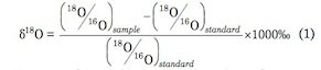
Because 16O is much more abundant than 18O, oxygen isotope ratios are expressed in units of “per mil” (per thousand) or “‰”. Higher values of this “oxygen isotope ratio” indicate an increased amount of 18O compared to 16O (relative to the standard), while a smaller value implies decreased amounts of 18O. δ18O values can be calculated for both calcium carbonate (CaCO3) and water, since both molecules contain oxygen.
Use of δ18O as a Climate Indicator
Under conditions of isotopic equilibrium, the δ18O value of calcium carbonate that precipitates out of water should depend only upon the temperature T and the δ18O value of the surrounding water (Grossman 2012; Shackleton and Kennett 1975).
Protists are tiny eukaryotic (having cells containing a nucleus) water-dwelling microorganisms. Marine protists called foraminifera (or forams) build shells (or tests) made of calcite, a form of calcium carbonate (CaCO3). At death, these shells become part of the ocean sediments drifting downward to the ocean bottoms. From the shell remains, oceanographers can determine the oxygen isotope ratio at different depths within the seafloor sediment cores. When graphed, these foraminiferal δ18Ocalcite values exhibit many “wiggles,” becoming larger and smaller with increasing depth (fig. 1).
Epstein et al. (1953) used least squares analysis to empirically determine a relationship between temperature T, the δ18O value of the calcite, and the δ18O value of the surrounding seawater for organically precipitated calcium carbonate at temperatures between about 7 and 30° C:
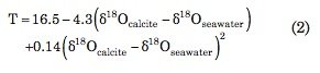
Other researchers have obtained similar equations for other temperature ranges and materials (Grossman 2012).
Although secular scientists have long viewed the foraminiferal oxygen isotope ratio as a climate indicator, the consensus interpretation of the variations in this variable has changed over the years. Cesare Emiliani, generally considered to be the founder of paleoceanography, argued that δ18Ocalcite was primarily a “paleothermometer”, and that more than 70% of the variation in δ18Ocalcite was due to temperature changes (Emiliani 1966). However, paleoclimatologist Nicholas Shackleton argued against this interpretation, noting that, if it were correct, it would have implied freezing of the oceans at times in the past (Shackleton 1967; Wright 2010). The consensus view now is that these variations are indicators more of changes in ice sheet volume than in temperature per se (Walker and Lowe 2007). High values of the oxygen isotope ratio within the sediments are thought to indicate times of greater ice volume (glacial intervals, or “ice ages”).
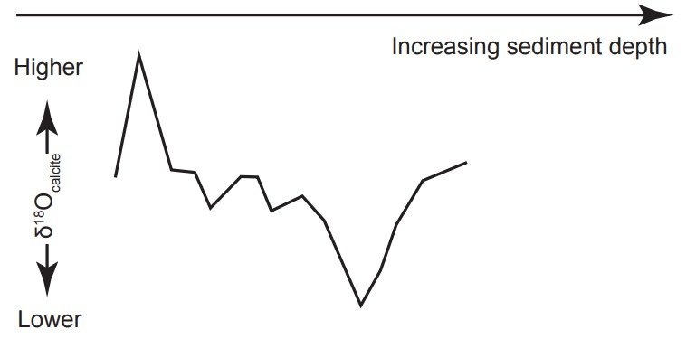
Figure 1. Secular scientists believe that maximum and minimum values in the “oxygen isotope ratio” indicate times of maximum and minimum glacial extent, respectively.
Upon reflection, this uncertainty in the interpretation of the δ18Ocalcite values is not surprising. Because δ18O values within the high latitude ice sheets tend to be much lower than typical oceanic δ18O values (about −35‰ compared to about 0‰), it is generally thought that the melting or growth of these large ice sheets could noticeably affect oceanic δ18O values (Wright 2010). Hence it seems reasonable that variations in global ice sheet volume could influence oceanic δ18O values, which is one of the two explicit variables affecting δ18Ocalcite values. But since δ18Ocalcite values also depend on temperature, and since larger ice sheets are also generally associated with lower temperatures, how does one de-convolve which part of the variation in δ18Ocalcite is a result of changes in temperature per se, and how much is a result of changes in ice volume? Moreover, temperatures depend upon local variations in time and space, even when global averages remain constant. How then, does one determine what part of the temperature is the result of a global average and how much is due to local temporal and spatial variations? Secular scientists claim to be able to infer how much of the changes in δ18Ocalcite is due to temperature and how much is due to changes in ice volume (e.g., Elderfield et al. 2012), but such claims are unwarranted due to their implicit, uncritical acceptance of the old-earth timescale, as well as the factors discussed further below.
The difficulty in separating how much of the δ18Ocalcite signal is due to temperature changes and how much is due to changes in global ice volume, even within a uniformitarian framework, is just one of many serious problems in attempting to use δ18Ocalcite values to infer past climates (Oard 1984).
Orbital Tuning
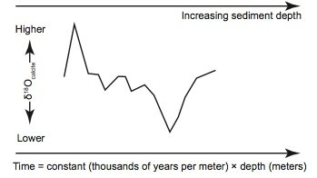
Figure 2a. The simplest possible “depth-age” model would assume that seafloor sediments at a given location have been deposited on the ocean floor at a perfectly constant rate throughout earth history and would (unrealistically) neglect possible compression and reworking of the sediments.
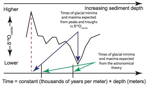
Figure 2b. However, if one assumes such a simplistic “depth-age” model, then the times assigned to extreme δ18Ocalcite values (indicating glacial maxima and minima) generally do not agree with the expectations of the astronomical theory.
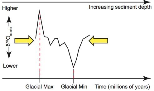
Figure 2c. However, secular paleoclimatologists can “explain” this disagreement by assuming that sedimentation rates for this section of the sediment core had been higher than average. This would cause these extreme δ18Ocalcite values to be farther apart than expected. Hence secular paleoclimatologists can “correct” for this higher-than-average rate by “compressing” the δ18Ocalcite signal in this part of the core.
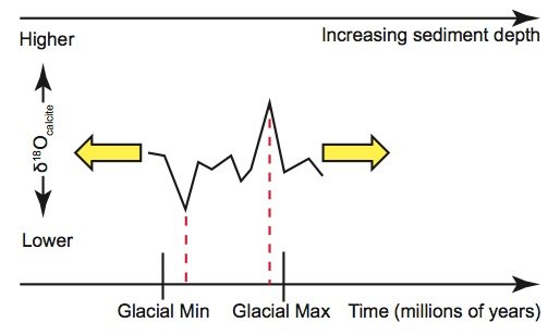
Figure 2d. Likewise, extreme δ18Ocalcite values in another section of the sediment core might be closer together than expected on the basis of a perfectly uniform sedimentation rate. Uniformitarians can “explain” this by assuming that these sedimentation rates were lower than average, which would place the extreme values closer together than expected. “Stretching” this section of the δ18Ocalcite signal brings the sediment ages into alignment with the expectations of the astronomical theory.
Even if one were to accept the premise that seafloor sediment δ18Ocalcite values are indeed global climate indicators, the construction of a “history” of earth’s climate still requires that dates be assigned to the climatic events associated with these oxygen isotope fluctuations. This requires a “depth-age” model that will assign an age to a given depth of seafloor sediment. The simplest possible “depth-age” model assumes that sediments at a given location have been deposited on the seafloor at exactly the same rate throughout earth history. In that case, the age of a given sediment layer is simply a constant multiplied by the layer’s depth, as measured from the position of the uppermost sediments (fig. 2a). However, even uniformitarian scientists do not believe that sedimentation rates have been that uniform. Likewise, they recognize that seafloor sediments are compacted after burial (Herbert 2010). Moreover, if one were to assume perfectly constant sedimentation rates, the ages assigned to the sediments would not in general agree with expectations from the astronomical theory (fig. 2b). So, despite their belief in “slow and gradual” geological processes, uniformitarian scientists believe that sedimentation rates have varied somewhat throughout earth history, with some times characterized by slightly higher sedimentation rates and other times characterized by slightly lower rates. Secular scientists are not bound by observations and feel free to select depth-age models that suit their purposes, and they use this fact in assigning dates to the seafloor sediments.
Remember that secular scientists believe that the astronomical theory “tells” them the times in the distant past that ice ages have occurred. Remember also that peak values in the δ18Ocalcite values are thought to indicate times of greatest ice cover ( “glacial maxima”), while minimal δ18Ocalcite values are thought to indicate minimal ice cover during the warmer “interglacials.” The orbital tuning method, in essence, uses the astronomical theory to assign the “correct” dates to these extreme δ18Ocalcite values. Secular researcher T. D. Herbert explains (Herbert 2010, p. 370):
Because the timing of orbital changes can be calculated very precisely over the past 30 My, and because their general character can be deduced for much longer intervals of geological time, orbital variations provide a template by which paleoceanographers can fix paleoclimatic variations to geological time. Paleoceanographers now commonly assign either numerical ages or elapsed time to sediment records by optimizing the fit of sedimentary variations to a model of orbital forcing, a process referred to as ‘orbital tuning’. [italics mine]
The orbital tuning method allows sedimentation rates to be varied, or “tuned,” in such a way that “glacial maximum” layers of sediment—those layers containing peak foraminiferal δ18Ocalcite values—will be deposited on the ocean floor at the approximate times demanded by the astronomical theory. There are several different mathematical approaches to the orbital tuning method, and these may involve techniques such as band-pass filtering or complex demodulation (Herbert 2010). However, in essence, orbital tuning allows secular scientists to selectively squeeze (fig. 2c) and expand (fig. 2d) different sections of the δ18Ocalcite signal in an accordion-like fashion so that maxima and minima δ18Ocalcite values are more-or-less aligned with the times demanded by the astronomical theory.
It should be noted that the often impressive correlations between various climatic variables and the astronomical theory are almost always obtained after the variables have been “tuned” by the astronomical theory.
Circular Reasoning
Of course, there is clearly a possibility for self-deception with this method. As noted by one researcher (Herbert 2010, p. 372), “The possibility clearly exists to produce a tuned sedimentary series that has been forced to resemble an orbital template by overenthusiastic correlation.”
In fact, two recent papers (Blaauw 2010; Blaauw, Bennett, and Christen 2010) dramatically illustrate the possibility for such self-deception. The authors of these papers demonstrated that it is possible to construct two random-walk time series with similar degrees of autocorrelation and to “match” similar features within the two series so that one series can be convincingly correlated with the other one—even though the two series are unrelated! If two unrelated randomly-generated time series can be convincingly correlated with one another, how can secular scientists be sure that they are not simply deceiving themselves when they correlate variations in δ18Ocalcite with purported variations in solar insolation over hundreds of thousands of years?
Secular scientists are aware of this possibility and attempt to remove some of the bias from the method. For instance, when determining possible sedimentation rates, they may devise programs that consider different possible alignments in order to obtain the best overall fit, while penalizing alignments that require extreme sedimentation rates or sudden changes in those rates (Lisiecki and Raymo 2005). However, as these methods implicitly assume that a best fit does exist, they never actually question the correctness of the astronomical theory.
Secular scientists use a number of “checks” or “constraints” on the method (Herbert 2010, p. 373) in an attempt to guard against the possibility of circular reasoning:
Orbital tuning is rarely applied to sediments without first considering independent age constraints from fossil events and paleomagnetic reversals. These provide a preliminary age scale and therefore a guide to approximate, time-averaged, sedimentation rates to be modified by orbital tuning.
But what are these constraints, and are they really independent?
An Independent Check?: Fossil Events
Since secular scientists claim that sedimentary layers were deposited slowly over millions of years, they argue that the fossils within these layers provide “snapshots” of life on earth at times in the “prehistoric” past. Index fossils are fossils that have been found only within relatively narrow ranges of sedimentary layers, and uniformitarians interpret this to mean that these organisms lived only within relatively brief windows of “prehistoric” time.
Uniformitarian scientists thus feel free to use these index fossils to “date” the sedimentary rocks in which they are found. But of course, this, in and of itself, does not yield “absolute” ages for the sediments or fossils. These “absolute” ages might be obtained by radioisotope dating, not of the fossils or the sediments themselves, but of volcanic rocks above and below the sedimentary layers “sandwiched” between them. Once an absolute age has been assigned to the stratum containing the index fossil, secular scientists then use that index fossil to date other sedimentary layers which also contain that same index fossil. In other words, secular scientists use the assumed evolutionary history of life in order to date the sedimentary rock layers (Ager 1983). This is what is meant by using “fossil events” or “faunal succession” to date the rocks.
Within a biblical worldview of course, the locations of these fossils tell us absolutely nothing about an alleged “prehistory” of millions of years, since most of the fossils were formed during the Genesis Flood. In fact, many “Lazarus taxa” have been discovered: index fossils found in layers outside of the range of strata in which they were previously found (Stanley 1998). This clearly demonstrates that previous attempts to use these index fossils for dating purposes were in error. And when one stops to think about it, how do we know that the same will not be true tomorrow for any supposed index fossil?
Furthermore, there is evidence that evolutionists have been unduly influenced by evolutionary expectations when assigning taxonomic names to different fossils. Nearly identical fossils have frequently been assigned different taxonomic classifications simply because they were found in different sedimentary layers (Werner 2008).
An Independent Check?: Paleomagnetic Reversals
The field of paleomagnetic stratigraphy endeavors to deduce information about earth’s past magnetic history from several different kinds of remanent magnetism.
Thermoremanent magnetization occurs when iron-containing minerals (such as magnetite, Fe3O4; hematite, Fe2O3, and ilmenite, FeTiO3) within volcanic rocks record the direction of the earth’s magnetic field (Garland 1979) at the time the rocks cool below the Curie temperature. The Curie temperature is the temperature below which a “paramagnetic” material with randomly oriented magnetic dipole moments becomes “ferromagnetic” or “magnetized,” having more strongly aligned magnetic dipole moments (Halliday, Resnick, and Crane 1992).
A second, unrelated process called detrital remanent magnetization occurs when magnetic grains within sediments align with the earth’s magnetic field during or shortly after deposition (Denham and Chave 1982).
Also, magnetic minerals can record the direction of the earth’s magnetic field as they are being formed from nonmagnetic minerals in a process called chemical magnetization (Garland 1979).
For earth scientists, thermoremanent magnetization is arguably the most informative of these three kinds of remanent magnetization, and it is thermoremanent magnetization found in seafloor volcanic rocks that played a large role in the development of the idea of seafloor spreading (Daintith 2005).
Both creation and uniformitarian scientists generally agree that earth’s magnetic field has “flipped” multiple times. Creation scientists believe these magnetic reversals occurred rapidly during the Genesis Flood (Humphreys 1990), while uniformitarian scientists generally believe that these reversals occurred slowly over thousands of years—despite the fact that secular scientists themselves have found evidence for extremely rapid magnetic reversals within volcanic rocks (Coe and Prévot 1989; Coe, Prévot, and Camps 1995). As new molten material comes up from the earth’s interior at the mid-ocean ridges, the current orientation of earth’s magnetic field is “recorded” by iron-containing minerals as the rock cools below the minerals’ Curie temperatures. This new seafloor spreads, with the older rocks located at progressively greater distances from the ridge. The boundaries between the “+” and “–” patterns in the volcanic rocks therefore indicate times at which the earth’s magnetic field reversed or flipped.
Although paleomagnetism is not a dating method per se, magnetic reversals could conceivably be used to assist in the dating of seafloor sediments if the reversals themselves can be dated. Uniformitarian scientists in the past have generally relied upon radioisotope dating methods, such as the potassium-argon (K/Ar) method, to do so. The most recent major magnetic reversal, the Matuyama-Brunhes reversal, is dated as having occurred 780,000 years ago (Pillans 2003). These magnetic reversals are viewed by secular scientists as especially important chronological “tiepoints” for the construction of a secular chronology (Agrinier, Gallet, and Lewin 1999; Channell et al. 2010), much in the same way that a biblical scholar would use important dates (such as dates for the Exodus) as “tiepoints” in the construction of a biblical chronology.
Creation scientists have long pointed out that there are serious problems with radioisotope dating methods, and all three of the main assumptions behind these methods are questionable (Vardiman et al. 2003). In addition to these fundamental problems with radioisotope methods, neither radioisotope nor paleomagnetic dating methods are truly independent.
“Good” and “Bad” Radioisotope Dates
Despite the popular perception that radioisotope dating methods yield absolute dates, the reality is quite different. Creationists will likely not be surprised to learn that the astronomical theory has been used to “adjust” or “calibrate” radioisotope dates. Herbert (Herbert 2010, p. 374) describes how K/Ar age assignments for the geomagnetic polarity timescale (GPTS) were judged by a team of secular scientists (led by Dutch stratigrapher Frits Hilgen) to be in need of “calibration” because they contradicted the astronomical theory:
Hilgen and co-workers recognized orbital forcing by a grouping of sapropels (dark, organic-rich beds) into units of ~100 and 400 ky by eccentricity modulation of precessional climate changes. Their resulting calibration of the GPTS yielded significantly greater ages for magnetic reversal boundaries than the previously accepted dates based on K/Ar radiometric age dating. After initial controversy, the ages proposed by Hilgen and others have largely been verified by recent advances in 40Ar/39Ar dating of volcanic ash layers at a number of magnetic reversal boundaries.
One of the “others” proposing an alternative timescale was Nicholas Shackleton. In 1990 he was the lead author on a paper (Shackleton, Berger, and Peltier 1990) that argued that the then-accepted age of 730,000 years for the Matuyama-Brunhes magnetic reversal (which was based upon K/Ar dating) should be revised upward to 780,000 years. Shackleton, Berger, and Peltier based their reasoning on the astronomical theory. Because the K/Ar dates were a little younger than those demanded by the astronomical theory, these K/Ar dates were revised upward. Likewise, the 40Ar/39Ar dates were deemed more accurate because they agreed with the astronomical theory. As we shall see later, this kind of reasoning is not isolated.
It should be noted that radioisotope dates have also been rejected because they contradicted evolutionary ideas about “faunal succession” (Lubenow 1995), which is another way of saying that evolutionary dogma trumped supposedly “scientific” dating methods.
So the expectations of both the evolutionary “story” and the astronomical theory have been allowed to overrule the supposedly “absolute” dates obtained from radioisotope dating methods. The circularity in such reasoning is obvious.
The 40Ar/39Ar Dating Method
The 40Ar/39Ar method (Merrihue and Turner 1966) is now viewed as a large improvement over the older K/Ar dating method and is thought to be capable of dating potassium-containing rocks or minerals of any age greater than a few thousand years (Jourdan, Mark, and Verati 2014). Uniformitarians have made much of the fact that the Ar/Ar method was used to apparently successfully date the AD 79 eruption of Mt. Vesuvius (Dalrymple 2000; Renne et al. 1997). However, this claim has been critiqued in the creation literature, and a case can be made that this 40Ar/39Ar age assignment was actually 72% higher than the true age (Overman 2010).
Although a detailed discussion of the 40Ar/39Ar method is beyond the scope of this paper, it should be noted that the method requires rocks or minerals of known age, age “standards” or “flux monitors,” in order to assign an absolute age to a rock or mineral of unknown age. The most common standard in use is the mineral sanidine from Colorado’s Fish Canyon Tuff (Jourdan, Mark, and Verati 2014).
In the Ar/Ar method, both the rock to be dated and the standards are bombarded for several days with fast neutrons from a nuclear reactor. As a result of this bombardment, stable 39K is converted into radioactive 39Ar. Because 39Ar has a half-life of 269 years, the amount of 39Ar resulting from this reaction may be safely assumed to be approximately constant during the time of the analysis (Faure and Mensing 2005).
The amount of 39Ar produced in this irradiation process depends upon the number of 39K atoms within the irradiated sample, the length of time for which the sample is irradiated, the neutron flux density (as a function of energy), and the neutron capture cross section for 39K. In actual practice, the energy spectrum of the incident neutrons and the neutron capture cross sections are not well known, which makes direct calculation of the number of resulting 39Ar atoms difficult. However, this difficulty is circumvented by combining the expression for this number of 39Ar atoms with the equation for the number of 40Ar atoms resulting from radioactive decay of 40K. A quantity called J, or the “irradiation parameter” is then defined. It is thought that J can be calculated for a flux monitor of known age without precise knowledge of the neutron energy spectrum and the neutron capture cross sections. After calculating these J values for the flux monitors within the reactor, these values of J are plotted as a function of position, and interpolation is then used to obtain the J value for the sample being dated (Faure and Mensing 2005).
Once J has been determined for the rock to be dated, it may be used, along with its ratio of radiogenic 40Ar compared to 39Ar, 40Ar*/39Ar, to obtain a calculated age for the rock.
Of course, it is the ratio of total 40Ar to 39Ar that is actually measured with a mass spectrometer. In order to obtain the ratio of radiogenic 40Ar to 39Ar, it is necessary to make a number of assumptions in order to estimate how much of the measured 40Ar is actually radiogenic. Also, it is necessary to correct for Ar isotopes that are produced in “cross reactions” resulting from interactions of neutrons with calcium, potassium, and chlorine in the sample. These assumptions and corrections are then used in conjunction with the sample’s J value to obtain a calculated age for the rock (Faure and Mensing 2005).
Calibration of 40Ar/39Ar Age Standards
There are a number of potential problems with this method, but of particular interest to this study is the manner in which the age of the standard is determined. Since the standard must also be a potassium-containing rock or mineral, one approach is to date the standard with the K/Ar method (Anonymous 2014). So in essence, Ar/Ar method is just an extension of the K/Ar method, and the K/Ar method is being used to calibrate itself!
In passing, it should be noted that it is fairly common for uniformitarian scientists to use one radioisotope dating method to calibrate another radioisotope dating method. For instance, uranium-thorium ages for corals have been used to calibrate the carbon-14 timescale (Bard et al. 1990). Of course, the fact that radioisotope dates need to be “calibrated” or “synchronized” (Kuiper et al. 2008; Renne, Karner, and Ludwig 1998) is a clear indication that such dates are not absolute, despite popular perception.
However, a second method is often used to date the age standards—the astronomical theory! This is a technique known as “intercalibration” (Renne et al. 1994), in which the ages assigned to sediments by the astronomical theory are used to constrain the ages assigned to volcanic rocks.
One should remember that radioisotope dates are necessary to assign ages to paleomagnetic reversals, which, according to Herbert (Herbert 2010) are supposed to act as independent “constraints” on the orbital tuning method. But at some point, secular scientist “lost sight” of this, and they began using the astronomical theory to calibrate their radioisotope dating methods!
Obviously, if the astronomical theory is being used to calibrate the age standards for the Ar/Ar dating method, then it is not really an independent “check” on the method.
Even a cursory literature search reveals that the use of the astronomical theory to “calibrate” dating methods is rampant in the historical sciences (Channell et al. 2010; Huang, Hesselbo, and Hinnov 2010; Meyers et al. 2012; Renne et al. 1994; Rivera et al. 2011; Shackleton, Berger, and Peltier 1990).
Square Pegs into Round Holes
Thus we see that “fossil events” and “paleomagnetic reversals” are not genuine independent checks on the orbital tuning method. Rather, both the evolutionary timescale and the astronomical theory are assumed to be true, and these assumptions are then used as criteria by which dating methods are judged to be “correct” or “incorrect.”
Despite this circular reasoning, however, the methods still contradict one another. A couple of examples follow.
First, in the late 1980s and early 1990s, scientists constructed a chronology for the last 500,000 years that presented a serious challenge to the astronomical theory (Winograd et al. 1992). This chronology was based upon oxygen isotope analysis and uranium-series dating of a calcite coating on the walls of the Devil’s Hole fault crack in the Nevada desert. This chronology actually had the penultimate (second-to-last) deglaciation occurring 140,000 years ago. This was problematic because, according to the astronomical theory, the increases in summer sunlight that would have caused this deglaciation occurred about 130,000 years ago. Hence, this new chronology has the second-to-last deglaciation occurring about 10,000 years before the increases in summer sunlight that were supposed to have caused it! Among paleoclimatologists, this is the so-called Termination II (T-II) “causality problem” (Shakun et al. 2011).
By the late 1990s, a team of geochronologists declared that the astronomical theory was indeed correct (Edwards et al. 1997), although, paradoxically, the Devils Hole chronology also appeared to be correct! Despite this declaration of victory for the Milankovitch theory, the issue does not appear to be settled. Papers addressing this problem are still being published, and “the causality problem remains a major focus of research” (Shakun et al. 2011, p. 1).
Second, it should be remembered that the most common age standard for the Ar/Ar dating method is Fish Canyon sanidine (FCs), and the age estimate for the FCs standard has been astronomically tuned (Kuiper et al. 2008) to about 28 million years. (Renne et al. 2010) then proposed an additional calibration for the Ar/Ar method. However, experts at the Columbia University Geochronology laboratory noted problems with their proposal (Hemming, Chang, and Tsukui, n.d.):
While the Renne et al. approach is cogent, the implied age of 28.305 Ma for Fish Canyon sanidine presents some clear problems. It pushes the 40Ar/39Ar [sic] age estimates for several important events to values that are significantly older than either U-Pb or astronomical estimates. For example, the implied 40Ar/39Ar age of the Bishop Tuff is already “too old” compared to astronomical calibrations of the Matuyama-Brunhes geomagnetic reversal . . . .
(Renne et al. 2010) also noted that their proposal led to other contradictions with the orbital tuning method. For instance, their re-calculated age for the Cretaceous/Tertiary boundary was about 279,000 years older than the age estimate for the boundary obtained by orbital tuning (Kuiper et al. 2008). They concluded that the difference was significant at the 95% confidence level. Likewise, the difference between their new age estimate for the FCs and the astronomically-tuned value was also significant at the 95% confidence level.
At this point, a review is in order. Remember that the date assigned by the K/Ar method to the Matuyama-Brunhes reversal was revised upward from 730,000 years to 780,000 years in order to agree with expectations of the astronomical theory (Shackleton, Berger, and Peltier 1990). Remember also that the good agreement between the astronomically-calibrated ages and the Ar/Ar dating method supposedly “confirmed” the accuracy of these astronomically-tuned dates (Herbert 2010). Then, the age assigned to the Fish Canyon sanidine (FCs) Ar/Ar dating standard was also calibrated to agree with the astronomical theory (Kuiper et al. 2008). But a logically “cogent,” and presumably more precise, re-calibration of the Ar/Ar dating method (Renne et al. 2010) led to another age estimate of the FCs that differed from the astronomically-tuned age for the FCs, as well as to a date for the Bishop Tuff that was in tension with the orbitally-tuned date for the Matuyama-Brunhes reversal. Likewise, this calibration led to a re-calculated date for the Cretaceous/Tertiary boundary that was also in tension with the orbitally-tuned date for that event. Even with all this manipulation, there are still disagreements between the dating methods! Of course, such contradictions are to be expected if the astronomical theory were simply wrong.
Seafloor Sediment Cores Used to Date Other Sediment Cores
The astronomical theory is used to date seafloor sediment cores, and these sediment cores are, in turn, used to date other sediment cores. For instance, (Pahnke et al. 2003) claimed to provide a 340,000 year chronology for the 36 m (118 ft) long MD97-2120 sediment core retrieved from Chatham Rise east of New Zealand. Between a depth of 6.8 and 10.6 m (22.3 and 34.7 ft), the age tie points used to construct the model ages for this sediment core were obtained by “tuning” its δ18O variations to δ18O variations in the MD95-2042 sediment core (located off the Portuguese coast). More discussion of this age model for the Chatham Rise core follows.
Dating of Ice Cores
Despite the apparent circular reasoning in these dating methods, one might object that timescales for the Greenland and Antarctic deep ice cores agree with expectations of the astronomical theory, thus validating these old-earth assumptions. As one might expect, however, the ages assigned to the ice cores are not independent, either.
Many people are under the impression that Antarctic and Greenland deep ice cores are dated simply by counting visible layers. This impression is erroneous, since visible layering is generally only present in the upper and middle sections of Greenland ice cores, as layering becomes indistinct at greater and greater core depths (Anonymous n.d.). Annual snowfall on the Antarctic plateau is generally too light (Palerme et al. 2014) to result in well-defined layers for the deep Antarctic cores (Oard 2005).
Furthermore, the weight of the overlying ice causes the ice to thin with increasing depth. Hence, a mathematical flow model is needed to assign an age to a given depth within the ice. Thus, flow models are used (sometimes in conjunction with “layer counting”) in order to date the ice cores. In fact, glacial expert W. S. B. Paterson acknowledged that ice flow models are actually the most common method of dating ice cores (Paterson 1991).
These flow models make a number of assumptions, including the assumptions that the high latitude ice sheets have been in existence for millions of years and have maintained more or less the same heights for all that time. In other words, the ice sheets are assumed to be in a near “steady state” of equilibrium. These assumptions naturally lead to extreme thinning of the lowermost layers of ice and vast age assignments.
However, the ice flow models do not simply assume an old earth, they also assume the validity of the astronomical theory. This is because the astronomical theory is used to calibrate the ice flow models! For instance, the timescale for Antarctica’s Vostok core was “tuned” (Waelbroeck et al. 1995, p. 113) to ensure that it agreed with the chronology derived from the seafloor sediments:
Taking advantage of the fact that the Vostok deuterium (δD) record now covers almost two entire climatic cycles, we have applied the orbital tuning approach to derive an age-depth relation for the Vostok ice core, which is consistent with the SPECMAP marine time scale. A second age-depth relation for Vostok was obtained by correlating the ice isotope content with estimates of sea surface temperature from Southern Ocean core MD 88-770.
Deuterium is a “heavy” isotope of hydrogen containing one proton and neutron. Since water molecules contain both oxygen and hydrogen, a deuterium isotope ratio may be calculated in a similar fashion to the oxygen isotope ratio. The SPECMAP (SPECtral MApping Project) marine time scale is the orbitally-tuned seafloor chronology constructed using oceanographic data collected during the 1980s. So secular scientists used orbital tuning to construct an ice core age-scale that agreed with the orbitally-tuned (!) age-scale for the seafloor sediments. Note that they also used seafloor sediment data to directly construct a second age-scale for the Vostok ice core. Other researchers have also used orbital tuning to obtain timescales for the Vostok ice core (e.g., Shackleton 2000).
But secular scientists might respond that other dating methods can be used to corroborate the ages assigned by these flow models. In particular, seasonal variations in the oxygen isotope ratio and volcanic reference horizons are thought to act as “checks” on the dates assigned by the flow models. However, such “checks” can generally only be used in the upper portions of the cores and can offer no real help in the dating of the deeper parts of the cores, which contain most of the alleged “time.” For instance, seasonal oxygen isotope variations in Greenland’s well-known GISP2 core disappeared at a depth of only 300 m (984 ft) (Meese et al. 1997), rendering them useless as a “check” on dates assigned to deeper sections of the core. Likewise, accurate historical dates for volcanic eruptions generally are only known for the last 300 years (Moore, Narita, and Maeno 1991), with a few large eruptions that can potentially be historically dated to no later than 2000 years ago (Meese et al. 1997).
Detailed critiques of the problems involved in the dating of the ice cores have already been presented in the creation science literature, as well as arguments for the youthfulness of the high latitude ice sheets (Oard 2004; Oard 2005). It should be noted that at “Ice Age” depths within the ice cores, higher amounts of dust are present (Paterson 1991), especially in the Greenland cores. Likewise, secular scientists have identified 700 sulfate volcanic signals in the portion of the GISP2 ice core (Zielinski et al. 1996) which creation scientists would date as from the post-Flood Ice Age, and these signals are believed to have originated from volcanic eruptions larger than historical eruptions known to have affected Northern Hemisphere climate. Evidence of greater volcanic activity in the deeper parts of the cores is consistent with the Creation-Flood Ice Age model (Oard 1990), which posits that the necessary summer cooling for the Ice Age was caused by large amounts of post-Flood volcanism.
Coming Full Circle: Using Ice Cores to Date Seafloor Sediments
As noted earlier, the “tie points” used in the construction of the chronology for the middle section of the MD97-2120 Chatham Rise seafloor sediment core were obtained by “tuning” δ18O variations within the core to δ18O variations within still another sediment core, the MD95-2042 core. However, the “tie points” for the lowest portion of the Chatham Rise core were obtained by tuning assumed sea surface temperatures to variations in the deuterium ratio of the Vostok ice core (Pahnke et al. 2003). In other words, the Vostok ice core was used to date the lower portion of this sediment core, even though the timescale for the Vostok core was obtained via orbital tuning (Shackleton 2000). Hence, the dating of the seafloor sediments and ice cores is truly a gigantic exercise in circular reasoning.
Conclusion
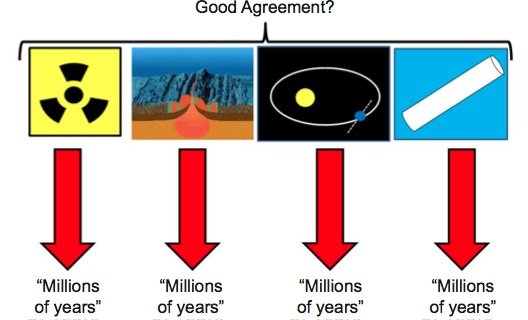
Figure 3a. The popular perception of various dating methods: the methods are independent of one another and yield “millions of years” because the earth really is unimaginably old. The “Magnetic Reversals” image (second from left) is a screen save of an animation produced by the U.S. Geological Survey that is in the public domain (commons.wikimedia.org/wiki File:Mid-ocean_ridge_topography.gif),
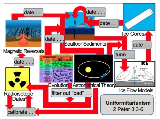
Figure 3b. The true relationships between the various “old earth” dating methods. The evolutionary timescale and the astronomical theory are assumed to be true and are used to date the seafloor sediments via the “orbital tuning” process. The seafloor sediment cores are then used to assist in the dating of other seafloor sediment cores, as well as to calibrate the ice flow models that ultimately assign dates to the deep Greenland and Antarctic ice cores. The ice cores are then used to date other seafloor sediment cores. These dating methods constitute a gigantic exercise in circular reasoning, and supposedly independent “checks” on the orbital tuning method, such as paleomagnetic reversals and or radioisotope dating, are not truly independent, as they too are influenced by old-earth assumptions. The “Magnetic Reversals” image was produced by the U.S. Geological Survey and is in the public domain (commons.wikimedia.org/wiki/File:Mid-ocean_ridge_ topography.gif), and the “Ice Flow Models” image was provided by Michael Oard (used with permission).
The apparent agreement between multiple, supposedly independent dating methods (fig. 3a) gives an undeserved aura of validity to old earth dogma. In reality, these methods are not independent of old earth assumptions, and the apparent agreement between these methods is the result of an enormous amount of circular reasoning (fig. 3b). Even with this circular reasoning, discrepancies and contradictions between the different methods do exist, although these contradictions are not well-known by the general public. Of course, underlying this entire network of circular reasoning is the assumption of uniformitarianism, against which the Apostle Peter warned us long ago (2 Peter 3:3–6).
For this reason, creation researchers should exercise extreme caution when attempting to use oxygen isotope seafloor sediment data to constrain post-Flood models of earth history, as these data have been manipulated to agree with the evolutionary, old earth paradigm. Although such use of these data may be possible, it should not be attempted without first conducting a thorough analysis of the raw oxygen isotope data as a function of depth and geographic location.
Creation researcher Marvin Lubenow (Lubenow 1995, p. 38) aptly summarized the manner in which dating methods are made to “serve” the evolutionary story: “In the dating game, evolution always wins.”
References
Ager, D. V. 1983. Fossil frustrations. New Scientist 100:425.
Agrinier, P., Y. Gallet, and E. Lewin 1999. On the age calibration of the geomagnetic polarity timescale. Geophysical Journal International 137, no. 1:81–90.
Anonymous. n.d. Using ice flow models for dating. Centre for Ice and Climate. Niels Bohr Institute. Retrieved from www.iceandclimate.nbi.ku.dk/research/flowofice/modelling_ice_flow/ice_flow_models_for_dating/ on May 9, 2014.
Anonymous. 2014. New Mexico Geochronology Research Laboratory. K/Ar and 40Ar/39Ar Methods: The 40Ar/39Ar Dating technique. Retrieved from geoinfo.nmt.edu/labs/argon/methods/home.html on May 7, 2014.
Bard, E., B. Hamelin, R. G. Fairbanks, and A. Zindler. 1990. Calibration of the 14C timescale over the past 30,000 years using mass spectrometric U-Th ages from Barbados corals. Nature 345, no. 6274:405–410.
Baumgardner, J. R. 1994. Runaway subduction as the driving mechanism for the Genesis Flood. In Proceedings of the Third International Conference on Creationism, ed. R. E. Walsh, pp. 63–75. Pittsburgh, Pennsylvania: Creation Science Fellowship.
Blaauw, M. 2010. Out of tune: The dangers of aligning proxy archives. Quaternary Science Reviews 36:38–49.
Blaauw, M., K. D. Bennett, and J. A. Christen. 2010. Random walk simulations of fossil proxy data. The Holocene 20, no. 4:645–649.
Channell, J. E. T., D. A. Hodell, B. S. Singer, and C. Xuan. 2010. Reconciling astrochronological and 40Ar/39Ar ages for the Matuyama-Brunhes boundary and late Matuyama Chron. Geochemistry, Geophysics, Geosystems 11, no. 12:1–21.
Coe, R. S. and M. Prévot. 1989. Evidence suggesting extremely rapid field variation during a geomagnetic reversal. Earth and Planetary Science Letters 92, no. 3–4:292–298.
Coe, R. S., M. Prévot, and P. Camps. 1995. New evidence for extraordinarily rapid change of the geomagnetic field during a reversal. Nature 374:687–692.
Cronin, T. M. 2010. Paleoclimates: Understanding climate change past and present. New York, New York: Columbia University Press.
Daintith, J. ed. 2005. Palaeomagnetism. Dictionary of physics, 5th ed. Oxford, United Kingdom: Oxford University Press.
Dalrymple, G. B. 2000. Radiometric dating does work! Reports of the National Center for Science Education 20, no. 3:14–19. Retrieved from ncse.com/rncse/20/3/radiometric-dating-does-work on April 24, 2014.
Denham, C. R. and A. D. Chave. 1982. Detrital remanent magnetization: Viscosity theory of the lock-in zone. Journal of Geophysical Research 87, no. B8:7126–7130.
Edwards, R. L., H. Cheng, M. T. Murrell, and S. J. Goldstein. 1997. Protactinium-231 dating of carbonates by thermal ionization mass spectrometry: Implications for Quaternary climate change. Science 276, no. 5313:782–786.
Elderfield, H., P. Ferretti, M. Greaves, S. Crowhurst, I. N. McCave, D. Hodell, and A. M. Piotrowski. 2012. Evolution of ocean temperature and ice volume through the mid-Pleistocene climate transition. Science 337, no. 6095:704–709.
Emiliani, C. 1966. Isotopic paleotemperatures. Science 154, no. 3751:851–857.
Epstein, S., R. Buchsbaum, H. A. Lowenstam, and H. C. Urey. 1953. Revised carbonate-water isotopic temperature scale. Bulletin of the Geological Society of America 64, no. 11:1315–1326.
Faure, G., and T. M. Mensing. 2005. Isotopes: Principles and applications, 3rd ed. Hoboken, New Jersey: John Wiley & Sons.
Garland, G. D. 1979. Introduction to geophysics: Mantle, core and crust, 2nd ed. Philadelphia, Pennsylvania: W. B. Saunders Co.
Glasby, G. P. 1978. Deep-sea manganese nodules in the stratigraphic record: Evidence from DSDP cores. Marine Geology 28, no. 1–2:51–64.
Grossman, E. L. 2012. Applying oxygen isotope paleothermometry in deep time. In Reconstructing earth’s deep time climate—The state of the art in 2012, Paleontological Society Short Course. The Paleontological Society Papers 18, ed. L. C. Ivany, and B. T. Huber, pp. 39–67.
Halliday, D., R. Resnick, and K. S. Krane. 1992. Physics, vol. 2, 4th ed. New York, New York: John Wiley & Sons.
Hayes, J. D., J. Imbrie, and N. J. Shackleton. 1976. Variations in the earth’s orbit: Pacemaker of the Ice Ages. Science 194, no. 4270:1121–1132.
Hemming, S., S. Chang, and K. Tsukui. n.d. Argon geochronology for the earth sciences, Columbia University. Retrieved from www.ldeo.columbia.edu/res/fac/argon/earthtime.html on May 9, 2014.
Herbert, T. D. 2010. Paleoceanography: Orbitally tuned timescales. In Climates and oceans, editor-in-chief J. H. Steele, pp. 370–377. Amsterdam, The Netherlands: Academic Press.
Huang, C., S. P. Hesselbo, and L. Hinnov. 2010. Astrochronology of the late Jurassic Kimmeridge Clay (Dorset, England) and implications for earth system processes. Earth and Planetary Science Letters 289, no. 1–2:242–255.
Humphreys, D. R. 1990. Physical mechanism for reversals of the earth’s magnetic field during the Flood, Proceedings of the Second International Conference on Creationism, vol. 2, ed. R. E. Walsh, and C. L. Brooks, pp. 129–142. Pittsburgh, Pennsylvania: Creation Science Fellowship.
Imbrie, J. 1982. Astronomical theory of the Pleistocene ice ages: A brief historical review. Icarus 50, no. 2–3:408–422.
Jourdan, F., D. F. Mark, and C. Verati. 2014. Advances in 40Ar/39Ar dating: from archaeology to planetary sciences—introduction. Advances in 40Ar/39Ar dating: from archaeology to planetary sciences, ed. F. Jourdan, D. F. Mark, and C. Verati. London, United Kingdom: The Geological Society of London Special Publications 378:1–8.
Kuiper, K. F., A. Deino, F. J. Hilgen, W. Krijgsman, P. R. Renne, and J. R. Wijbrans. 2008. Synchronizing rock clocks of earth history. Science 320, no. 5875:500–504.
Lisiecki, L. E. and M. E. Raymo. 2005. A Pliocene-Pleistocene stack of 57 globally distributed benthic δ18O records. Paleoceanography 20, no. 1:PA1003.
Lubenow, M. L. 1995. The pigs took it all. Creation 17, no. 3:36–38.
Luyendyk, B. P. 2014. Oceanic crust. Encyclopaedia Britannica online. Retrieved from www.britannica.com/EBchecked/topic/424497/oceanic-crust on June 3, 2014.
Meese, D. A., A. J. Gow, R. B. Alley, G. A. Zielinski, P. M. Grootes, M. Ram, K. C. Taylor, P. A. Mayewski, and J. F. Bolzan 1997. The Greenland Ice Sheet Project 2 depth-age scale: Methods and results. Journal of Geophysical Research 102, no. C12:26411–26423.
Merrihue, C. and G. Turner. 1966. Potassium-Argon dating by activation with fast neutrons. Journal of Geophysical Research 71, no. 11:2852–2857 .
Meyers, S. R., S. E. Siewert, B. S. Singer, B. B. Sageman, D. J. Condon, J. D. Obradovich, B. R. Jicha, and D. A. Sawyer. 2012. Intercalibration of radioisotopic and astrochronologic time scales for the Cenomanian-Turonian boundary interval, Western Interior Basin, USA. Geology 40, no. 1:7–10.
Milanković, M. 1941. Canon of insolation and the Ice-Age problem (in German). Belgrade, Serbia: Special Publications of the Royal Serbian Academy, vol. 132.
Moore, J. C., H. Narita, and N. Maeno. 1991. A continuous 770-year record of volcanic activity from east Antarctica. Journal of Geophysical Research 96, no. D9:17353–17359.
Oard, M. J. 1984. Ice Ages: The mystery solved? Part II: The manipulation of deep-sea cores. Creation Research Society Quarterly 21, no. 3:125–137.
Oard, M. J. 1990. An ice age caused by the Genesis Flood. El Cajon, California: Institute for Creation Research.
Oard, M. J. 2004. Ice cores vs the Flood. TJ 18, no. 2:58–61.
Oard, M. J. 2005. The frozen record. Santee, California: Institute for Creation Research.
Oard, M. J. 2011. The remarkable African Planation Surface. Journal of Creation 25, no. 1:111–122.
Overman, R. 2010. Evaluation of the Ar/Ar dating process. Creation Research Society Quarterly 47, no. 1:23–30.
Pahnke, K., R. Zahn, H. Elderfield, and M. Schulz. 2003. 340,000-year centennial-scale marine record of Southern Hemisphere climatic oscillation. Science 301, no. 5635:948–952. The measured δ18O values from this core, as well as the methods used to obtain the core’s age model, have been summarized and archived at ftp.ncdc.noaa.gov/pub/data/paleo/contributions_by_author/pahnke2003/pahnke2003.txt. Retrieved on May 8, 2014.
Palerme, C., J. E. Kay, C. Genthon, T. L’Ecuyer, N. B. Wood, and C. Claud. How much snow falls on the Antarctic ice sheet? The Cryosphere Discussions 8:1279–1304. Retrieved from www.the-cryosphere-discuss.net/8/1279/2014/tcd-8-1279-2014-print.pdf on May 9, 2014.
Patrick, K. 2010. Manganese nodules and the age of the ocean floor. Journal of Creation 24, no. 3:82–86.
Paterson, W. S. B. 1991. Why ice-age ice is sometimes “soft.” Cold Regions Science and Technology 20:75–98.
Pillans, B. 2003. Subdividing the Pleistocene using the Matuyama-Brunhes boundary (MBB): An Australasian perspective. Quaternary Science Reviews 22:1569–1577.
Renne, P. R., A. L. Deino, R. C. Walter, B. D. Turrin, C. C. Swisher III, T. A. Becker, G. H. Curtis, W. D. Sharp, and A. Jaouni. 1994. Intercalibration of astronomical and radioisotope time. Geology 22, no. 9:783–786.
Renne, P. R., W. D. Sharp, A. L. Deino, G. Orsi, and L. Civetta. 1997. 40Ar/39Ar dating into the historical realm: Calibration against Pliny the younger. Science 277, no. 5330:1279–1280.
Renne, P. R., D. B. Karner, and K. R. Ludwig. 1998. Absolute ages aren’t exactly. Science 282, no. 5395:1840–1841.
Renne, P. R., R. Mundil, G. Balco, K. Min, and K. R. Ludwig. 2010. Joint determination of 40K decay constants and 40Ar*/40K for the Fish Canyon sanidine standard, and improved accuracy for 40Ar/39Ar geochronology. Geochimica et Cosmochimica Acta 74, no. 18:5349–5367.
Rivera, T. A., M. Storey, C. Zeeden, F. J. Hilgen, and K. Kuiper. 2011. A refined astronomically calibrated 40Ar/39Ar age for Fish Canyon sanidine. Earth and Planetary Science Letters 311, no. 3–4:420–426.
Shackleton, N. 1967. Oxygen isotope analyses and Pleistocene temperatures re-assessed. Nature 215:15–17.
Shackleton, N. J. 2000. The 100,000-year Ice-Age cycle identified and found to lag temperature, carbon dioxide, and orbital eccentricity. Science 289, no. 5486:1897–1902.
Shackleton, N. J. and J. P. Kennett. 1975. Paleotemperature history of the Cenozoic and the initiation of Antarctic glaciation: Oxygen and carbon isotope analyses in DSDP Sites 277, 279, and 281. In Initial reports of the Deep Sea Drilling Project, vol. 29, ed. S. M. White, pp. 743–755. Washington, D.C.: U.S. Government Printing Office.
Shackleton, N. J., A. Berger, and W. R. Peltier. 1990. An alternative astronomical calibration of the lower Pleistocene timescale based on ODP Site 677. Transactions of the Royal Society of Edinburgh: Earth Sciences 81, no. 4:251–261.
Shakun, J. D., S. J. Burns, P. U. Clark, H. Cheng, and R. L. Edwards. 2011. Milankovitch-paced Termination II in a Nevada speleothem? Geophysical Research Letters 38, no. 18:L18701.
Stanley, G. D., Jr. 1998. A Triassic sponge from Vancouver Island: Possible holdover from the Cambrian. Canadian Journal of Earth Sciences 35, no. 9:1037–1043.
Twidale, C. R. 1982. Planation surfaces—Theory and reality. In Perspectives in geomorphology, vol. 1, ed. H. S. Sharma, pp. 63–82. New Delhi, India: Naurang Rai, Concept Publishing Co.
Vardiman, L. 1996. Sea-floor sediment and the age of the earth. El Cajon, California: Institute for Creation Research.
Vardiman, L. 2003. Hypercanes following the Genesis Flood, In Proceedings of the Fifth International Conference on Creationism, ed. R. L. Ivey Jr., pp. 17–28. Pittsburgh, Pennsylvania: Creation Science Fellowship.
Vardiman, L., and W. Brewer. 2011. A Well-Watered Land: Numerical Simulations of a Hypercyclone in the Middle East. Answers Research Journal 4:55–74.
Vardiman, L., S. A. Austin, J. R. Baumgardner, E. F. Chaffin, D. B. DeYoung, D. R. Humphreys, and A. A. Snelling. 2003. Radioisotopes and the age of the earth. In Proceedings of the Fifth International Conference on Creationism, ed. R. L. Ivey Jr., pp. 337–348. Pittsburgh, Pennsylvania: Creation Science Fellowship.
Waelbroeck, C., J. Jouzel, L. Labeyrie, C. Lorius, M. Labracherie, M. Stiévenard, and N. I. Barkov. 1995. A comparison of the Vostok ice deuterium record and series from the Southern Ocean core MD 88–770 over the last two glacial-interglacial cycles. Climate Dynamics 12:113–123.
Walker, M. and J. Lowe. 2007. Quaternary science 2007: A 50-year retrospective. Journal of the Geological Society 164, no. 6:1073–1092.
Werner, C. 2008. Evolution: The grand experiment, vol. 2. Green Forest, Arkansas: New Leaf Press.
Winograd, I. J., T. B. Coplen, J. M. Landwehr, A. C. Riggs, K. R. Ludwig, B. J. Szabo, P. T. Kolesar, and K. M. Revesz. 1992. Continuous 500,000-year climate record from vein calcite in Devils Hole, Nevada. Science 258, no. 5080:255–260.
Wright, J. D. 2010. Cenozoic climate—oxygen isotope evidence. In Climates and oceans, editor-in-chief J. H. Steele, pp. 316–327. Amsterdam, The Netherlands: Academic Press.
Zielinski, G. A., P. A. Mayewski, L. D. Meeker, S. Whitlow, and M. S. Twickler. 1996. A 110,000-yr record of explosive volcanism from the GISP2 (Greenland) Ice Core. Quaternary Research 45, no. 2:109–118.