
The views expressed in this paper are those of the writer(s) and are not necessarily those of the ARJ Editor or Answers in Genesis.
Abstract
The present article is the third in a series of papers intended to identify and, where possible, to quantify the key sources of the heat inevitably released during the Genesis Flood. In contrast with the first two papers, which are concerned mainly with the thermal history of the oceans, it considers the thermal consequences of vapour canopy models of the pre-Flood earth and of the onset of the Flood. Such models were developed in the last decades of the twentieth century by creationist authors who proposed that the pre-Flood earth possessed an atmosphere characterised by a high-altitude water vapour canopy which would have collapsed at the onset of the Flood, thereby providing a proportion of the water involved in the Flood. Here we find that the vapour canopy idea arose from outside mainstream biblical scholarship, apparently with the long-age catastrophist Isaac Newton Vail, who in turn attributed it to philosopher Immanuel Kant. Other strands of thought seem likely to have contributed, but their origin is not entirely clear. Our appraisal of the biblical and scientific arguments used to support the development of the idea into computationally tractable models of the pre-Flood atmosphere has found that the biblical arguments are not compelling. Furthermore these models fail scientifically, mainly because they predict a pre-Flood environment which would have been too hot for life except where the canopy water content was far too small to contribute significantly to the floodwaters.
Keywords: Vapour canopy; pre-Flood earth; atmosphere; greenhouse effect; temperature profile.
Introduction
The catastrophic global Flood at the time of Noah (described in Genesis 7 and 8) must have generated an enormous quantity of heat, thus raising the question of how environmental temperatures were kept within limits. This article is the third in a series aiming to identify, and where possible to quantify, the sources of Flood heat in order to provide boundary conditions and guidelines for creation scientists seeking to explain how the necessary cooling was accomplished.
The first article, Part 1 (Worraker 2018), considered boundary conditions relevant to modelling the earth’s thermal history including its internal temperature field, past and present ocean temperatures, surface heat flows and its inventory of heat-producing radionuclides. Of the various indicators of past ocean temperatures in current use, Part 1 dealt only with the oxygen isotope ratio (18O/16O) in fossil shells and in ice, expressed as the δ18O value. Part 2 (Worraker 2019) considered other widely-used indicators, viz. (1) Mg/Ca (magnesium/calcium) ratios in calcite fossil shells, notably those produced by foraminifera; (2) trace element methods, e.g. Sr/Ca and Li/Mg ratios, with particular application to corals; (3) biomolecular index methods, of which three are now commonly used in marine temperature reconstructions; (4) the carbonate clumped isotope index.
The present article, Part 3, considers a different type of Flood heat problem, namely the thermal consequences of vapour canopy models of the pre-Flood earth and of the onset of the Flood. Such models were developed in the second half of the twentieth century by creationist authors who proposed that the pre-Flood earth possessed an atmosphere characterised by a high-altitude water vapour canopy. Within the present-day creationist movement this concept was first articulated by Whitcomb and Morris (1961), and the popularity of canopy theories among young-earth creationists, notably in the 1970s and 1980s, is probably due in the first instance to the influence of Whitcomb and Morris’s (1961) book because of its comprehensive scope and its role in launching the movement. However a much earlier version of a watery canopy enveloping the earth was proposed in a long-age catastrophist framework by Isaac Newton Vail (1902, 1905, 1912). Vail’s ideas influenced Whitcomb and Morris (1961) and, through them, subsequent creationist authors including notably Dillow (1981) and Vardiman (1986). Vail himself attributed the canopy idea to the influential “Age of Enlightenment” German philosopher Immanuel Kant (1755); see also Bixler (1986). In pursuing the exercise advocated by Wise (2018, 693) of reconstructing “the intellectual history of creationism”, we first consider Jerome’s legacy, followed by the ideas of Kant and Vail as significant intellectual background to the development of canopy theories within contemporary young-earth creationism.
The single most comprehensive modelling exercise based on the concept of a pre-Flood vapour canopy surrounding the earth is represented by Joseph Dillow’s (1981) book, the prime focus of this review. The next three sections therefore review the literature on Flood-related canopy models in chronological order thus: (1) publications up to 1980; (2) Dillow’s (1981) book, the first part dealing mainly with his Scriptural arguments and the second with his scientific arguments and modelling; and (3) subsequent publications. Our conclusions follow. An Appendix is included which addresses technical issues arising from Dillow’s (1981) book, and not, to the knowledge of the present author, considered elsewhere.
Earliest References: Jerome, Kant and Vail
The first reference to anything remotely suggesting a canopy surrounding the pre-Flood earth comes from Jerome (c. 347–420 AD), the chief translator of the Latin Vulgate, who in commenting on Genesis 1 describes a crystalline (probably icy) expanse or canopy above the cherubim in Ezekiel’s inaugural vision (Ezekiel 1:22, 23, 25, 26). The relevant passage in Jerome’s Latin original (Migne 1845, 659) is:
Inter cælum et terram, medium exstruitur firmamentum; et juxta Hebraici sermonis έτυμολογίαν cælum, id est, SAMAIM, ex aquis sortitur vocabulum: et aquæ quæ super cælos sunt, in laudes Dei separantur. Unde et in Ezechiele Propheta, Crystallum super Cherubim videtur extensum (Ezech. 1), id est, compactæ et densiores aquæ.
The key clause here is Crystallum super Cherubim videtur extensum (Ezech. 1), id est, compactæ et densiores aquæ, which roughly translates as “ice appeared stretched out above the cherubim (Ezekiel 1), that is, compressed, denser waters” (see also Bixler 1986). Jerome, and indeed the translators of the Septuagint, were doubtless influenced by the Greek concept of the heavens as a series of concentric hard spheres, which was already in circulation in the sixth century B.C. (Younker and Davidson 2011). This legacy is seen in the translation firmament in the 1611 King James (and related versions) of Genesis 1:6–8 where the Hebrew text has rāquîa and the Septuagint στερέωμα. Both the Latin firmamentum and the Greek στερέωμα imply something solid, but in context this is not a good rendering of rāquîa; its basic meaning is something “extended” or “spread out” (Calvin 1554; Poole 1685; Keil and Delitzsch 1869; Leupold 1942; Kaiser 2013). Fouts (2015, 91) has noted that the concept of a solid dome over the earth, also popular in many ancient cultures, has provided “plenty of foundation for misunderstanding what the text is actually saying.” The concept of a pre-Flood vapour or liquid water canopy around the earth is clearly not attributable to Jerome: relatively few twentieth-century canopy theorists have considered a canopy in solid form.
Isaac Newton Vail (1840–1912) was a Quaker “learned in mathematics, astronomy, Latin and Greek” (The Velikovsky Encyclopedia 2019). Vail (1912, vi–vii) attributed the origin of the basic canopy idea to Immanuel Kant (1724–1804), but notes that after introducing the idea Kant then advised against it. Kant (1755) seems to have had a special fascination for Saturn and its rings. He says (chapter 5, 1:303):
Could we not imagine that the Earth once had a ring like Saturn? . . . But what a stock of lovely explanations and consequences such an idea presents us with! A ring around the Earth! What a beautiful sight for those created to inhabit the Earth as a paradise; what a comfort for those on which nature smiles from all sides! But this is nothing compared with the confirmation such a hypothesis can borrow from the chronicle of the story of creation and which is no small recommendation for applause for those who believe they are not desecrating but rather confirming the honour of revealed religion when they make use of it to give the excesses of their wits some prestige. The waters of the firmament mentioned in Moses’ description has already caused the interpreters some effort. Could one not use this ring to help to get oneself out of this difficulty? Without a doubt this ring consisted of watery vapours, and in addition to the advantage it was able to provide the first inhabitants of the Earth, there is the additional one of having it break when required so that floods could punish the world that had made itself unworthy of such beauty.
Having further elaborated his vision of the Flood, notably the introduction of the rainbow as a memorial sign, Kant (1755) concludes (chapter 5, 1:304):
The similarity of the shape of this memorial sign with the event it signified could commend such a hypothesis to those who are devoted to the dominant tendency of bringing the miracles of revelation into the same system as the ordinary laws of nature. I consider it more advisable completely to forgo the fleeting applause such correspondences might arouse for the true pleasure that arises from the perception of regular connections when physical analogies support each other to designate physical truths.
Thus having introduced the idea that the earth might once have been enveloped by a ring-derived vapour canopy which subsequently collapsed to produce the Genesis Flood, Kant retracts it because he sees it as a “god of the gaps” explanation. He prefers a thoroughly mechanistic understanding of the Flood. This may be seen as an early expression of Kant’s rationalism, characterised, despite references in his writings to grace and revelation, by an autonomous natural order with no place for grace or divine revelation (Schaeffer 1968).
Vail (1912, v) cites the purpose of the original 1874 edition of his own book thus:
. . . to show that the Deluge of Noah, and all the “Ice Ages” were caused by the progressive and successive collapse of great world-canopies of aqueous vapor, which were the last remnants of a Saturn-like Ring System or a Jupiter-like “Cloud Ocean,” sent to the terrestrial skies when the earth was in its molten stage. In that edition it was also shown that earth-canopies were competent to produce all the tropic eras the earth ever saw. It was also pointed out that world-canopies trending poleward tended to mass themselves in the polar heavens, and fall in the Arctic and Antarctic regions as vast avalanches of snow.
Thus Vail believed that the earth had possessed a Saturn-like ring system which degenerated into a series of world-embracing vapour canopies, which then collapsed via a succession of catastrophic snowfalls in the polar regions. Much of the evidence Vail cites in support of his theory is based on ancient mythologies, viewed as fossilised collective memories of spectacular meteorological and geological phenomena. Vail (1902) refers to a number of biblical themes and names, including Eden, the “tree of life and death” (sic), Leviathan (Job 41:1–34; Psalm 74:13–14; Isaiah 27:1), the Fall of Lucifer (Isaiah 14:12), Ophir (1 Kings 9:28, 10:11 etc), and the Great Red Dragon (Revelation 12:3–4). His book The Deluge and its Cause (Vail 1905) seeks to uphold the Mosaic account of the Genesis Flood, which he attributes to the last of a series of global canopy collapse events. However Vail (1912, 25) believed that his postulated vapour canopy had persisted for millions of years before its final demise. Although Vail is biblically literate, his treatment of Scripture does not qualify as serious biblical scholarship. Fig. 1 shows Vail’s conception of a vapour canopy enveloping the earth just prior to the Genesis Flood, while fig. 2 (based on Figure 4, Vail 1912) shows a sketch of its development as ring material supposedly flowed earthwards.
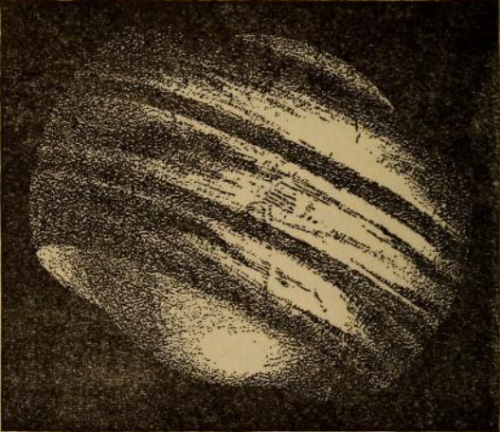
Fig. 1. Woodcut portrayal of Isaac Vail’s conception of “. . . the earth as it existed before the flood surrounded by a vapour canopy which caused perpetual summer; there was no rain, no sun, no moon, no rainbow, no storms or winds; no seasons, and man lived far longer than now. When this canopy fell as the DELUGE, the physical condition of the earth changed, and man’s environment was greatly modified.” (Vail 1905, frontispiece, 6).
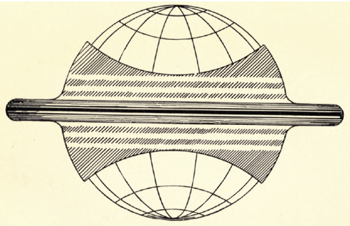
Fig. 2. A copy of Figure 4 in Vail (1912), depicting Vail’s conception of material from the earth’s postulated primordial ring system flowing earthward to become a canopy. Part of the original caption says: “An edge view of the Earth’s Annular System with its innermost ring having reached the atmosphere in its slow and gradual descent spreading from the equator to the poles. Revolving rapidly around the earth, it is thrown into bands, belts and lines as it forms into a canopy such as the planets Saturn and Jupiter have to-day. I want the reader to note particularly these linear formations and recognize the extremely slow lateral motion toward the poles where all canopies must end their career.” Vail refers this stage of his postulated canopy development to Job 26:7.
Intriguingly, Saturn’s rings (fig. 3) do produce a “ring rain” (Connerney 2013; O’Donoghue et al. 2013, 2019) falling continuously into the planet’s atmosphere. This consists of sub-micron sized ice particles which have become electrically charged either by photoionization or by exposure to dense plasma produced by micrometeorite impacts. These charged particles then flow along magnetic field lines and reach Saturn in mid-latitude regions. Their arrival facilitates charge-exchange reactions which locally reduce the density of H3+ ions in Saturn’s upper atmosphere, thus causing a detectable local reduction in H3+ infrared emission. However none of this provides a genuine physical analogy to Vail’s conception of the formation of an earth-enveloping vapour canopy produced by the disintegration of a Saturn-like ring system.
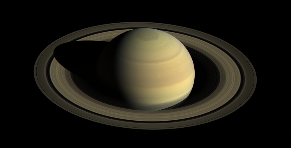
Fig. 3. Saturn and its rings imaged from the Cassini spacecraft in April 2016, using Cassini’s wide-angle camera at a distance of approximately 3,000,000 km (1,864,000 mi) from the planet and at an elevation of about 30° above the ring plane. Saturn’s equatorial diameter is approximately 120,540 km (75,000 mi). Image Credit: NASA/JPL-Caltech/Space Science Institute. Image source: https://photojournal.jpl.nasa.gov/catalog/PIA21046.
From the relevant writings of both Kant and Vail we therefore conclude that the concept of a vapour canopy enveloping the pre-Flood earth, which does not seem to have been invoked by Bible scholars through the first 1,900 years of Christian history, arose from outside faithful mainstream Bible scholarship. Given this background, it is noteworthy that vapour canopy proponents from 1961 onwards have occasionally leaned towards identifying the vapour canopy concept with the teaching of Scripture itself, an unjustified hermeneutical approach (Hodge 2019; Sarfati 2010; Wieland 1989, 2010); examples are noted in the following sections.
Vapour Canopy Literature up to 1980
An early brief reference to a pre-Flood vapour canopy is given by Rehwinkel (1951), who notes it as one of three possible theories proposed to explain his understanding of the earth’s antediluvian climate as uniformly warm, a conclusion based on the observations of Price (1923). Rehwinkel states (12) that (1) the canopy would have produced a temperature of 72ºF (= 22.2ºC), though he does not say how this figure was obtained or where exactly it would have applied, and that (2) the canopy, which would have collapsed at the onset of the Flood, would have been the chief source of the floodwaters. He proposes that during the pre-Flood period the canopy would have intercepted sunlight and thereby protected people and animals from its damaging effects, notably “the aging of living things” and “decay and fermentation”. Although Rehwinkel (1951) was clearly dependent on Price’s (1923) geological observations, he did not glean the idea of a pre-Flood vapour canopy from Price, who did not believe that there had been such a canopy (Wise 2019). Instead, Rehwinkel (1951, 12) makes a rather cryptic reference to a publication by Johannes Riem1, but it has not been possible at the time of writing to trace this item.
As already noted, Whitcomb and Morris (1961) strongly espoused the concept of a pre-Flood vapour canopy. Their first reference to “the waters above” (9) treats these waters as a major source of Flood rain: Presumably, then, the ocean basins were fractured and uplifted sufficiently to pour waters over the continents, in conjunction with those waters which were above the “firmament” (expanse) and which poured down through the “windows of heaven”.
Subsequently Whitcomb and Morris (1961, 77) state:
But if we accept the Biblical testimony concerning an antediluvian canopy of waters (Gen. 1:6–8, 7:11, 8:2, II Peter 3:5–7), we have an adequate source for the waters of a universal Flood.
This statement apparently equates the authors’ own interpretation with the teaching of Scripture itself (cf. Hodge 2019; Sarfati 2010). Whitcomb and Morris (1961) also ignore the priority of the breakup of “the fountains of the great deep” in the biblical description of the onset of the Flood in Genesis 7:11, where the order is probably significant (Barrick 2008, 268; Batten et al. 2017a, 169–170). They offer no justification for their interpretation of the above passages, nor any quantitative information beyond a rough estimate of the water content of earth’s present atmosphere, viz. the equivalent of about 2 in (5 cm) of rain (121), with a smaller estimate suggested in a footnote. In a section describing conditions in the antediluvian period of earth history, they state (215):
The waters “above the firmament” seem to imply more than our present clouds and atmospheric water vapor, especially since Genesis 2:5 implies that during this time rainfall was not experienced on the earth . . . . The upper waters did not, however, obscure the light from the heavenly bodies and so must have been in the form of invisible water vapor. Such a vast expanse of water vapor would necessarily have had a profound effect on terrestrial climates and therefore on geological activity.
This assumes that the “no rain” condition in Genesis 2:5 still applied long after Creation Week. No justification is offered for the claimed transparency of a vapour canopy. As for climatic conditions, Whitcomb and Morris (1961, 240–242) subsequently elaborate their view, stating that their proposed vapour canopy would “cause a uniformly warm, temperate climate around the earth”, lead to an absence of atmospheric turbulence and of high-altitude condensation nuclei, and would produce a very gentle hydrological cycle based on the mist of Genesis 2:6. They acknowledge (253–255) that it would have warmed the earth via a greenhouse effect, but offer nothing quantitative. The attractiveness of a vapour canopy is explained thus (256) in referring to “a substantial increase in the water vapor content of the upper atmosphere”, but note their well-advised caution at this point:
And this, of course, is exactly what we have seen the early chapters of Genesis to imply, in the references to the “waters above the firmament.” We feel warranted, therefore, in suggesting such a thermal vapor blanket around the earth in pre-Pleistocene times as at least a plausible working hypothesis, which seems to offer satisfactory explanation of quite a number of Biblical references and geophysical phenomena.
The “geophysical phenomena” mentioned here are the warm, temperate conditions inferred from the geological record to have existed generally across the pre-Flood earth (Price 1923; Rehwinkel 1951; Whitcomb and Morris 1961, 243–249). Various effects of the removal of the proposed canopy after the Flood are also suggested by Whitcomb and Morris (1961), including extreme latitudinal temperature variations resulting in great air movements and climatic zones (287), and more penetration of earth’s atmosphere by radiation, gas and dust from space (287). They also suggest (374–375) that there would have been (1) much less 14C in the pre-Flood atmosphere than today because of the shielding effect of the vapour canopy and (2) an enhanced level of atmospheric tritium production by the interaction of neutrons with deuterium in the water molecules2 because of the high level of water vapour there, thus explaining the (claimed) excess 3He in the atmosphere. The general post-Flood decline in human lifespan is attributed to the increase in harmful radiation from space resulting from the disappearance of the canopy, which is supposed to have protected people and animals against somatic and genetic radiation damage (Whitcomb and Morris 1961, 399, 404–405).
That such a canopy would have had a profound climatic effect has been confirmed by subsequent quantitative analysis (Dillow 1981, 1983; Rush and Vardiman 1990; Vardiman 2003; Vardiman and Bousselot 1998): in fact all reasonable scenarios proposed hitherto involving more than a trivial quantity of water vapour in the model canopy and using reliable infrared absorption data indicate an overwhelming greenhouse effect, not what Whitcomb and Morris (1961) had in mind!
Udd (1975) argues that Genesis 1:6–8 refers to a canopy of liquid water above the atmosphere (in his view rāquîa = atmosphere). He cites 2 Peter 3:5,6 as implying that two bodies of water existed at the time of the Flood, and takes as given that the canopy disappeared at the onset of the Flood. Udd argues that the Greek word meaning water is used three times in these verses, of which two must mean liquid water, implying that the third usage must also refer to liquid water. However, he does not say which instance of the word has a questionable meaning, and not all commentators interpret them in this way. Lucas and Green (1995, 132), for example, speak of “. . . a bewildering range of options for translators” with regard to 2 Peter 3:5. Lucas and Green (1995, 132–133) also note that the literal translation of the beginning of 2 Peter 3:6 is “by means of which . . .”, where the word translated “which” is of plural form in the Greek original. They suggest that it may well refer to the word of God and to water, which gives a very coherent sense to the whole passage (vv. 1–13). Thus v. 6 may not be referring to a combination of the waters mentioned in v. 5, and indeed those waters could refer to one and the same body of water viewed from different perspectives. Udd (1975) also argues that Psalm 148:4, which seems to suggest that the “waters above the heavens” still existed in the psalmist’s time, refers to a creation context, and that it constitutes an example of poetic licence; he does not accept that Psalm 148:6 necessarily implies that the canopy is permanent. Some of Dillow’s (1981) biblical arguments for the existence of a pre-Flood vapour canopy derived from a primordial liquid water canopy are explicitly based on Udd’s arguments.
Strickling (1976) argues against the vapour canopy model. His point is that if “waters above the firmament” (Genesis 1:7) refer to a vapour canopy, then creation of “lights in the firmament of the heavens” (Genesis 1:14, 17) cannot refer to the sun, moon, and stars. This simple argument can be articulated in other ways; Dillow’s (1981) counterargument is considered below.
Kofahl (1977) argues that provision of a substantial part of the floodwaters either from a vapour canopy or other extraterrestrial sources of water or ice is incompatible with the known laws of physics—divine intervention would be needed. He considers the following issues: light transmission; high atmospheric pressure; unbearable temperatures and more. Kofahl notably assumes a canopy mass equivalent to 1000 ft (305 m) of water, giving an excess atmospheric pressure of 29.5 bar. He also analyses models involving a spherical shell of ice in space, ice orbiting the earth and an icy space impactor, demonstrating (should it be necessary!) that none will work. He later suggests a canopy holding 6 in (15 cm) of water to give a greenhouse climate in the created world. However he offers no explanation for the Flood, which he treats as an essentially supernatural phenomenon. Kofahl suggests that the “waters above” in Genesis 1:7 mean liquid water in the original.
In a series of three articles in Creation Research Society Quarterly, Dillow (1977, 1978a, 1978b) covers several technical aspects of the vapour canopy model he was developing at the time. Dillow (1977) considers the visibility of stars through the canopy; this is reproduced practically verbatim in Chapter 9 of his book (Dillow 1981), which is discussed below. Dillow (1978a) assesses the effect of the canopy on human longevity, material largely reproduced in Chapter 5 (146–182) of Dillow (1981), and Dillow (1978b) considers mechanical and thermodynamic characteristics of the canopy model. The material in this last paper is reproduced in more fully developed, quantitative form in Chapter 5 of Dillow (1981).
Westberg (1979) proposes a huge hollow crystalline ice sphere surrounding the earth from Creation Week Day 2 (Genesis 1:6–8), formed by water exploding to steam from a hot surface (Westberg 1980) and composed of radially-pointing ice crystals supposed to act like optic fibres. This ice canopy was supposedly 19,000 mi (30,600 km) thick, stretching from altitude 3,000 mi (4,800 km) to 22,000 mi (35,400 km). It then melted locally, disrupted and fell to earth as Flood rain. Before the Flood no solar heat would have reached the earth, which was supposedly heated from below. Morton (1980) offers a series of very obvious physical objections to this proposal; in reply, Westberg (1980) merely adds a few explanatory comments. To this reviewer Westberg’s proposal makes no sense, scientific or otherwise, and does not contribute meaningfully to serious Flood-related literature; it is noted here only for completeness.
Morton (1979), aware of contemporary development of a vapour canopy model by Joseph Dillow, presents an analysis of atmospheric temperatures under a vapour canopy assuming radiative equilibrium; the overall heat balance of the earth, subject to solar heating, is included. He considers a range of values of the quantity of water contained in the canopy, and different albedo (reflectance) values for the earth. He deduces that the only combination that would allow clouds to form (as had been suggested by Dillow) was 12 in (30 cm) of precipitable water in the canopy and an albedo of 0.9; in contrast, present-day observations of earthshine (the moon’s “ashen light”) give an average global albedo for the earth very close to 0.3 (Goode et al. 2001). Morton further argues that the presence of clouds would give even higher temperatures at the surface because the earth’s outgoing infrared radiation would be absorbed more strongly by the cloud droplets than by vapour, and less energy would therefore escape to space. He concludes that a vapour canopy would keep the earth too hot for life unless it was so lightweight that it would contribute very little of the water required for the Flood.
Joseph Dillow’s (1981) Vapour Canopy Model: Appraisal of Scriptural Basis
Several Scripture references have been invoked by creationist authors in support of the vapour canopy concept (e.g. e.g. Bixler 1986; Dillow 1979, 1981; Humphreys 1978; Rush 1990; Rush and Vardiman 1990; Whitcomb and Morris 1961). These include: (1) Genesis 1:6–8, which speaks of “the waters above the firmament”; (2) Genesis 2:5–6, which notes the absence of rain in the context of man’s creation, the ground being watered by a mist instead. This is taken to imply a climate very different from today’s; (3) Genesis 2:25, which is also taken to imply a warmer climate than today’s; (4) Genesis 8:22, which may suggest that the familiar cycle of “cold and heat” did not exist before the Flood; (5) Genesis 9:8–17, which describes the covenant of the rainbow, again possibly hinting at the absence of rain before the Flood; (6) Dillow (1979, 1981) interprets Psalm 148:4 as referring back to the created order (Genesis 1:6–8) on the premise that the Psalm naturally divides into two halves, vv. 1–6 and 7–14 respectively, the first referring to Creation Week and the latter to the Psalmist’s day. Dillow (1979, 1981) makes use of most of these passages: we consider his detailed arguments below.
Dillow (1981, chapters 2 and 3) argues for his “Water Heaven Theory” as the best interpretation of the relevant Scriptures. In these chapters the emphasis is on establishing that the “waters above the firmament” or “waters above the expanse” (Genesis 1:7) constituted a liquid water ocean above the atmosphere. He subsequently argues that this was instantly transformed into a vapour canopy, the centrepiece in his portrayal of the pre-Flood world.
He says (222, first paragraph):
For this reason, we propose that when God lifted up the deep from the surface of the earth and arched it over the ancient atmosphere, He instantly turned those waters into vapor form (superheated transparent steam) and established them in a pressure-temperature distribution that would not require miracles to maintain. The only basis for assuming this switch is that there is no indication in the Bible that these waters were maintained miraculously, we assume that God maintained them according to the laws of nature that are known today and that He Himself had established.
The second paragraph begins:
We readily admit that Genesis does not teach the existence of a pre-Flood vapor canopy. Moses simply says that God placed a canopy of liquid water above the ancient atmosphere. However, if scientific laws today existed then, it is necessary that God turned that water into vapor, even though Moses does not tell us that He did this.
In summary, Dillow (1981) acknowledges that his proposed pre-Flood vapour canopy is not directly taught by Scripture, but rather is based on his understanding of “the waters above” in Genesis 1:7 and the assumption that natural laws were in operation thereafter. Returning to chapters 2 and 3 in Dillow (1981), we consider his main arguments for the existence of a liquid water ocean above the atmosphere on Day 2 of Creation Week:
Clouds or a literal liquid ocean? Many commentators interpret “the waters above” as clouds (e.g. Benson 1857; Calvin 1554; Gill 1746–17633; Henry 1706; Keil and Delitzsch 1869; Leupold 1942; Poole 16854); Fouts (2015, 93, footnote 164) rejects the “heavenly ocean” interpretation. According to Dillow (1981, 50–51) the Genesis text (1:6) describes the division in the middle of the waters as a division in the waters of the deep of Genesis 1:2. He also says that there is no word in Genesis 1 corresponding to the translation cloud(s), whereas several such words are available in Hebrew. Dillow notes that the primary meaning of the preposition translated “above” is “upon” or even “beyond”, arguing that alternatives such as “in” or “within” do not do justice to the text; he cites Young (1964, 90, footnote 94) in his support.
However, the sun, moon, and stars are said in Genesis 1:14, 15 and 17 to have been placed in the expanse of the heavens. Thus Dillow’s argument based on the preposition above seems to prove too much; with regard to the expanse or atmosphere the prepositions above and in probably represent an observer’s perspective. Others have made very similar points (Strickling 1976; Whitelaw 1983). Dillow (1979) argues against this understanding, insisting that in the Genesis 1 account of creation, the work of Days 1–3 was primarily to give form to the earth, while in Days 4–6 God was filling the earth appropriately, such that the above relating to the waters in Gen. 1:7 is to be taken in a “literal mechanistic sense”, while the in relating to the sun, moon and stars in Genesis 1:14, 15 and 17 is to be taken as “observer true”. However Dillow’s (1979) division of the chapter into two parallel sets of three days is either ignored (e.g. Calvin 1554; Fouts 2015; Henry 1706; Kidner 1976; Leupold 1942) or rejected (e.g. Keil and Delitzsch 1869; Young 1964) by many interpreters. Although Dillow does not subscribe to the Framework Interpretation of Genesis 1, which is critiqued by McCabe (2008), his analysis follows similar lines. Thus Dillow’s choice of senses in which to read the prepositions above and in looks like special pleading.
Furthermore Dillow’s (1981, 56–57) insistence that the expanse was created as a division within the waters of the deep, implying that the “waters above” must have been in the form of a heavenly ocean, does not necessarily support his canopy theory since these waters could have turned into vapour (Dillow’s own proposal, noted above) or into clouds (composed of water droplets or ice particles or both), or first into vapour and then into clouds, or a mixture of the two in proportions varying in space and time; the biblical data is insufficient to distinguish between these scenarios. Dillow (1981, 240–246) himself invokes a deep cloud layer at the base of the canopy in an attempt to evade the unbearably hot surface conditions predicted by the cloud-free version of his model, but does not say when this cloud layer is supposed to have formed; in view of Genesis 1:31 this probably had to be in Creation Week. This is somewhat ironic, given Dillow’s rejection of the “clouds” interpretation of “the waters above” in Genesis 1:6-8.
Luther (1544a, 63–64) throws an interesting sidelight on the interpretation of Genesis 1:6–8:
We now come to the work of the second day, where we shall see in what manner God produced out of this original rough undigested mist or nebulosity, which he called “heavens,” that glorious and beauteous “heaven” which now is, and as it now is; if you except the stars and the greater luminaries. The Hebrews very appropriately derive the term shamayim the name of the heavens from the word mayim which signifies “waters.” For the letter schin is often used in composition for a relative, so that shamayim signifies “watery,” or “that which has a watery nature . . . And experience teaches that the air is humid by nature.”
Thus Luther sees the original deep of Genesis 1:2 as misty rather than distinctly liquid, notes the etymological connection in Hebrew between the expanse of heaven and its watery origin, and attributes a watery or humid nature to the atmosphere. Gill (1746–1763) also notes the etymology of the Hebrew word shamaim (sic) for the heavens, which he takes to indicate that there are “waters in the clouds of heaven.”
At this point it is worth digressing briefly to consider an alternative strand of interpretation of “the expanse” (rāquîa) and “the waters above” (mayim) in Genesis 1:6–8, viz. that “the expanse” refers to extraterrestrial space, and “the waters above” refers to cosmic waters in some form. This view is currently gaining popularity among creation scientists. For example, Johnson (1987) identifies the rāquîa with space in a wide range of contexts, but his ideas do not seem to have been followed up by others. Humphreys (1994a, 1994b)5, who rejects the interpretation of the waters above as clouds, treats them in his “white hole” cosmology as the raw material from which the elements were supposedly created (an idea expressly rejected by Keil and Delitzsch 1869), and in an alternative cosmological model as an extremely massive shell of ice enclosing the entire observable universe (Humphreys 2007). A similar role for the waters above was considered in Hartnett’s (2007, 94) cosmology, but the latter treats them as existing in the form of icy objects in the outer solar system. This general approach (i.e. rāquîa = space) is considered favourably by Faulkner (2016; 2018) and by Hebert (2017). However, the Hebrew word mayim (waters), notably in Genesis 1:6–7 and in Psalm 148:4, refers specifically to liquid water (as noted by Dillow 1981; Udd 1975), which conflicts with interpretations requiring this word to mean ice. Some earlier interpreters indeed view rāquîa as referring to the whole space above the earth (e.g. Calvin 1554), sometimes expressly including the starry heavens (e.g. Gill 1746–1763; Henry 1706; Poole 1685), and sometimes even as far as the “third heaven” or “heaven of heavens” (cf. Deuteronomy 10:14; 1 Kings 8:27; Nehemiah 9:6; 2 Corinthians 12:2 etc), e.g. Gill (1746–1763) and Henry (1706). However before the twentieth century interpretations of this kind were not used to develop physical cosmologies or, returning to the main theme of this article, to construct Flood models. They are not, and were not intended to be, directly relevant to the source of the floodwaters or to the heat deposited in the Flood.
Dillow (1981, 59–61) further argues for his “water heaven” interpretation of Genesis 1:6–8 by reference to 2 Peter 3:5–6; here he follows Udd’s (1975) argument noted and addressed above, viz. that the Greek word meaning water is used three times in these verses, of which two must mean liquid water, concluding that the third usage must also refer to liquid water. Dillow (1981, 104–108) also argues (again following Udd 1975) that Psalm 148:4, which seems to suggest that the “waters above the heavens” still existed in the Psalmist’s time, refers to a creation context; he sees it as an example of poetic licence. This again reads like special pleading. Dillow further notes the contrast between the “waters above the heavens” in v. 4 and the clouds in v. 8. Although his understanding of Psalm 148:4, in which “the waters above the heavens” refers to a now-vanished primordial high-altitude liquid ocean, seems exegetically possible, it is not convincing. Almost all other interpreters read Psalm 148:4 straightforwardly as referring to the present (e.g. Benson 1857; Calvin 1557; Gill 1746–1763; Henry 1706; Hodge 2019; Keil and Delitzsch 1871; Poole 1685). It is noteworthy that none of the earlier interpreters, who were not biased by the need to defend a particular theory, saw these waters as having ceased to exist. In summary, while Dillow argues his case cogently, he has limited support from other commentators and his insistence on the location and form of “the waters above” is partially self-refuting. There is no compelling biblical or scientific reason to suppose that a primordial high-altitude liquid water canopy would necessarily have turned into vapour rather than into clouds or varying proportions of vapour and cloud; Dillow’s “vapour only” choice turns out necessarily to involve a cloud base for the canopy.
The primordial watering of the earth. Another major argument used by Dillow (1981, 77–93) in support of his vapour canopy theory is based on Genesis 2:5-6, the key statements being (2:5, KJV)
. . . for the LORD God had not caused it to rain upon the earth . . .
and (2:6)
But there went up a mist from the earth, and watered the whole face of the ground.
Dillow (1981, 77–78) argues that the absence of rain would have been a natural consequence of a vapour canopy above the atmosphere, but admits that few commentators had come to this conclusion. Given that the next mention of rain (Heb. māṭar) occurs in Genesis 7:4 in connection with the Flood, and that God instituted the rainbow as a sign of his covenant of mercy toward the earth and every living creature (including people and animals) after the Flood (Genesis 9:8–17), Dillow infers a global climate between Creation Week and the Flood much quieter than today’s climate, i.e. negligible temperature differentials, minor wind movements and no rain (78). Rush (1990) follows Dillow’s lead in his view of the pre-Flood earth.
However the only necessary implications of the statements in Genesis 2:5–6 are: (1) the absence of certain types of plants, (2) the absence of rain, and (3) watering of the ground by a mist, all before the creation of man. Since plants were created on Day 3 and mankind on Day 6 of Creation Week, these conditions may have lasted for only three days. Furthermore conservative estimates of the time interval between Creation Week and the Flood, based on the genealogy in the Masoretic text of Genesis 5, exceed 1,600 years, an improbably long time for such conditions, notably the absence of rain, to persist. The rivers watering Eden (Genesis 2:10–14) after man’s creation may or may not have been typical of much of the primordial earth’s surface, but would probably have needed rain to replenish their water sources, at least regionally; mist (Genesis 2:6) would seemingly not have been adequate. We naturally infer that the mist of v. 6 had been replaced by the rivers of Eden, the latter participating in a hydrological cycle involving rain. Lisle (2019) argues similarly against a long-lasting rain-free climate. In contrast, Humphreys (1978), whom Dillow (1981, 282) cites in his support, expands Dillow’s vision of the pre-Flood climate by proposing, from his understanding of a number of (mostly) Old Testament Scriptures, that the earth’s outer core serves as a high-pressure, high-temperature water source, which regularly produced the mist of Genesis 2:6 through a global system of “super-geysers”. Humphreys also proposes that this source burst forth violently when “the fountains of the great deep” (Genesis 7:11) opened at the onset of the Flood, and is still in existence. Humphreys defends his idea scientifically by saying (146) “. . . there are no experimental data that the writer knows of which does not fit into the hypothesis of a water core.” However there seems to have been no follow-up in subsequent creationist literature, and no geological or geophysical evidence has since come to light which supports Humphreys’ idea in its original form.
The covenant of the rainbow. Commentators are divided as to whether the institution of the covenant of the rainbow after the Flood (Genesis 9:9–17) coincided with the first occurrence of a rainbow, or whether it was an existing phenomenon invested with special significance at a critical moment in history. Dillow (1981, 96) argues strongly that in the case of the sun, moon and stars (Genesis 1:14–18) and of the mark on Cain (Genesis 4:15), the first mention coincides with the assignment of significance, and that the rainbow constitutes a parallel case. However this is an argument from silence, an inherently poor way of reasoning. He further argues that institutions such as baptism and the Lord’s Supper are invalid analogies because they are “done by man and made by man” (96), whereas the rainbow is made by God alone. This ignores the fact that baptism and the Lord’s Supper, together with circumcision, the Passover and Old Testament blood sacrifices, were all instituted at the Lord’s command. Dillow (1981, 97) also argues that Genesis 9:13 speaks of putting or setting the rainbow in the sky rather than appointing it as a sign, implying that it was a new phenomenon; however he acknowledges that the same Hebrew word can mean appoint (e.g. Numbers 14:4; 1 Kings 2:35). Dillow’s view is supported by Luther (1544b), Keil and Delitzsch (1869) and by Leupold (1942), and is followed by Rush (1990). Calvin (1554, 217) takes the opposite view, speaking of Moses’ words as describing an act of consecration of an existing phenomenon:
I think the celestial arch which had before existed naturally, is here consecrated into a sign and pledge; and thus a new office is assigned to it . . .
Calvin thus sees the covenant of the rainbow as giving reassurance to people who may have otherwise, because of their experience or awareness of the global Flood itself, feared that another overwhelming flood was imminent when they saw deep cloud masses, rain and a rainbow. In his view it served as a sign of divine favour towards men. Benson (1857); Henry (1706); Lisle (2019); Sarfati (2010) and Whitelaw (1983) view it similarly.
Thus there seems to be no clear consensus among commentators on whether the rainbow had existed before God designated it a token of his covenant of mercy towards man and the whole creation. However, if we accept Dillow’s (1981) understanding that natural laws controlled atmospheric conditions between Creation Week and the Flood, it is difficult to see how a primordial, high-altitude vapour canopy could have lasted largely intact for a globally rain-free period of more than 1,600 years. Indeed, as indicated in the following section, Dillow’s modelling of pre-Flood environmental conditions leads to the near-certainty of rainfall during this period.
Other relevant Scriptures. Dillow (1981, 98–101) understands Genesis 8:22 to imply that seasonal climate involving extremes of hot and cold did not exist prior to the Flood. He dismisses the idea that Genesis 1:14 implies climate-related seasons, asserting that this verse refers to seasons as time markers only (99). Rush (1990) follows him in taking this view. However “seedtime and harvest” (Genesis 8:22) does seem to have been known before the Flood (Genesis 4:3), and the cycle of “day and night” certainly was known from Creation Week (Genesis 1:5; 1:14–19). Thus to argue that seasonal cold and heat were unknown until after the Flood reads like special pleading, and as another argument from silence.
Vardiman (1986) notes from Genesis 3:7–8 that Adam and Eve were initially naked. He sees this as evidence that the climate in Eden was “a tropical paradise”, which he links to the “no rain” conditions characterised by mist as the chief aboveground source of water in Genesis 2:5–6. Rush and Vardiman (1990) also cite Genesis 2:25 as evidence of warm climatic conditions everywhere on the primordial earth. However the climatic conditions (possibly) implied in these verses may only have applied locally in Eden, the geographical focus of the Genesis 2 narrative. Certainly when Adam and Eve were expelled from the Garden of Eden they began to wear clothing (Genesis 3:21), and subsequently lived in a harsher environment (Genesis 3:17–21) than they had known before, and all this long before the Flood. The biblical data are insufficient to establish the conditions required by Dillow’s theory, viz. that the earth as a whole was a “tropical paradise” for most of the time interval between Creation Week and the Flood.
Dillow (1981) not only discusses at considerable length the Scriptural evidence for a pre-Flood vapour canopy, but also cites a range of ancient mythological accounts from across the world which seem to refer to both a water heaven and to a global flood. His rationale is that the latter represent corrupted but genuine memories of historical realities recorded in Genesis. He also gives good reasons for doubting Sir James Frazer’s dismissal (Frazer 1918) of the Genesis account of the Flood as mythological and of any genuine link with reality in world mythology.
Joseph Dillow’s (1981) Vapour Canopy Model: Appraisal of Scientific Aspects
As for scientific evidence in favour of his theory, Dillow (1981, 138–139) begins by outlining ten predictions which, in his judgment, naturally follow: (1) A greenhouse effect; (2) A high present-day concentration of 3He; (3) Increased (pre-Flood) atmospheric pressure; (4) Shielding from cosmic radiation; (5) A global flood; (6) Volcanic ash mixed with ice; (7) A sudden and permanent temperature drop in the polar regions; (8) Fewer meteorites in pre-Flood strata; (9) Residual amounts of water in the stratosphere today; (10) A changed appearance of the heavenly bodies.
From his interpretation of Genesis 8:22 Dillow (1981, 98–101) believes that before the Flood there were no seasons as we know them (i.e. summer and winter), which implies that the earth would then have had a very small axial tilt6. His model involves a vapour canopy holding the equivalent of 12.19 m, or 40 ft, of precipitable water, enough to supply 40 days’ and nights’ worth of rain falling at a rate (suggested by Dillow) of 0.5 in (12.7 mm) per hour. Although this is a large amount of water it would clearly contribute very little to the overall floodwaters (Genesis 7:17–20); Dillow’s model, even in its design, comes nowhere near explaining the main source of the floodwaters. Significantly, perhaps, he ignores the priority of the “fountains of the great deep” over the “floodgates of heaven” in Genesis 7:11 and 8:2; however, as noted earlier, according to Barrick (2008, 268) the order in these verses “suggests that the fountains were the primary source of water that flooded the earth”.
The starting-point of Dillow’s modelling of the pre-Flood atmosphere, a variant of the “Emden model” (Dillow 1981, 226), employs a detailed multiwavelength radiation calculation of the corresponding atmospheric pressure and temperature profiles. He makes the following assumptions: (1) incoming solar radiation at today’s average level; (2) no clouds; (3) ten times today’s value of ozone (O3); (4) three times today’s value of carbon dioxide (CO2). Dillow rejects Morton’s (1979) analysis because the latter neglects the wavenumber dependence of albedo and absorption. Dillow’s (1981) model gives a surface temperature of 314°C (234) and a surface pressure of 2.18 bar; the latter figure is based on the mass of the current atmosphere plus the mass assumed for the canopy water content. The calculation giving these results was criticized by Morton (1982) because of an incorrect unit conversion, leading to T4 values 100 times too small. The same calculation with Morton’s correction included would thus give a surface temperature of 1417 K, or 1144ºC if radiation in the wavenumber interval 5.24 × 10⁵ to 5.54 × 10⁵ m-1 (or wavelength interval 1.805-1.908 μm) alone were considered. Dillow (1983) accepted this criticism.
Even the conditions resulting from Dillow’s (1981) uncorrected calculations are literally “too hot for comfort”; Dillow’s model is thus indefensible without modification. To salvage his modelling approach he argues (234) for the development of convection cells above the canopy base (at about 10.6 km or 6.6 mi altitude), condensation and the consequent formation of a deep cloud layer. This would significantly change the tropospheric radiation balance, and Dillow infers that the surface would be cooler than in the absence of clouds, and that the troposphere would be characterised by a temperature inversion. Dillow (1981, 235) states that in this model the canopy base temperature in the presence of convection and consequent cloud formation is 244°C at the poles. In the same context (235) he suggests that canopy “jet streams” will aid the redistribution of heat towards the poles. To demonstrate this scenario he offers a 1D, 3-layer model of the troposphere (depicted in Dillow 1981, Figure 7.2, 242, and reproduced in fig. 4 here) based on radiation balance between the cloud base, the tropospheric layers and the earth’s surface; solar heating is not explicitly included, and the radiation is treated as “grey” such that its properties are wavelength-independent. The resulting atmospheric temperature profile is shown in fig. 5 (which reproduces Figure 7.3, 243 in Dillow 1981): note the deep cloud layer between troposphere and vapour canopy. Dillow’s model of a cloud-topped troposphere is considered in detail in the Appendix, where it is shown to be incorrectly constructed. If set up correctly it simply gives the same temperature for the troposphere and surface as for the cloud base, viz. 100ºC; there is no tropospheric temperature inversion. Dillow (1981, 244) suggests that a multiwavelength model would do better: however the Appendix also shows that even in this case the temperature would be the same in the troposphere and on the earth’s surface as at the cloud base. It still fails to provide a solution to his basic heat problem. Dillow further argues (245–246), contrary to Morton, that the clouds proposed for keeping the surface temperature at reasonable levels would have dissipated at night, allowing people to see the stars (he refers to Genesis 1:14–19). However without quantitative modelling of the key processes it is not possible to settle this dispute. More importantly,
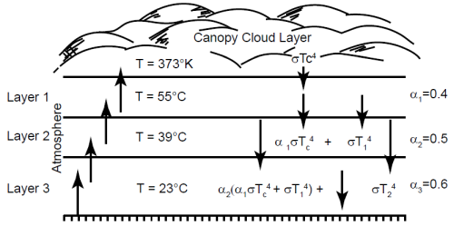
Fig. 4. Reproduction of Figure 7.2 from Dillow (1981, 242) showing a schematic of the lower part of his “cloud canopy” model.
Dillow has not demonstrated that his postulated canopy-base clouds, to which he assigns a huge vertical depth of about 10 km (6 mi) (see fig. 5), would not regularly, perhaps daily, produce large amounts of rain, most probably in the form of heavy thunderstorms. Since, as noted earlier, his postulated atmospheric conditions would probably have been in force since Creation Week, his model as presented seems to have led to pre-Flood conditions very different from his original perspective. The “no rain” condition certainly looks untenable.
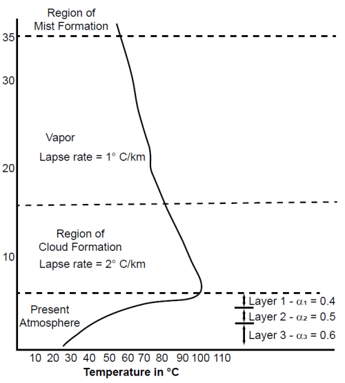
Fig. 5. Reproduction of Figure 7.3 from Dillow (1981, 243) showing the vertical temperature profile in his pre-Flood model atmosphere with clouds at the base of the vapour canopy.
Dillow’s vapour canopy model is questionable in several other ways, mostly in scientific terms:
1. Dillow’s (1981, 250–258) discussion of the stability of the pre-Flood atmosphere in terms of Taylor vortices is misleading and irrelevant. Taylor vortices represent the form of instability of the flow between rotating coaxial cylinders when the inner cylinder exceeds a critical angular velocity which depends on the dimensions of the system and the viscosity of the fluid between them (Chandrasekhar 1961; Taylor 1923). It is a purely dynamical instability arising from an adverse distribution of angular momentum, i.e. where the so-called Rayleigh criterion is violated7. In the absence of thermal effects a planetary atmosphere will rotate in synchrony with the planet, and the Rayleigh criterion is naturally satisfied. This would certainly be expected to apply for the earth from Creation Week onwards irrespective of the details of its atmosphere. Dillow thus rightly acknowledges (254) that the atmosphere would have been created in a state of dynamic equilibrium such that “the angular velocity of the inner rim of the canopy would be equal to the angular velocity of the surface of the earth”. However Dillow’s concept of an inner rim to the canopy, implying that it behaved like a solid wall (as shown in his Fig. 7.6, 252), is inapplicable in this context. The atmosphere/ canopy interface would not have been solid, and the discussion in terms of flow between solid cylinders is irrelevant to the earth’s atmosphere. Furthermore Dillow (254) mistakenly regards today’s high-altitude jet streams as evidence that the Taylor number of the atmosphere is above its critical value, thereby implying that he believes the jet streams to be evidence of Taylor instability. Dillow (1981, 253–255) cites John Burkhalter, an atmospheric physicist, in support of his understanding of atmospheric dynamics in terms of Taylor instability. However Dillow (1981, 255, footnote 55) subsequently seems to doubt that the global-scale averaged meridional circulations characterising today’s atmosphere really are Taylor vortices, while still entertaining the false idea that the vapour canopy had once fulfilled the role of an outer cylinder:
However, it may be questionable that these cells as they are constructed today are Taylor vortices as Burkhalter suggests. A similar cell pattern has been produced in laboratory atmospheric simulations based on thermal differences between the poles and the equator by Rossby and Fultz. Furthermore, computer simulated climate models have predicted a similar flow pattern without any reference to concentric cylinders and a moving fluid in between; see Battan, pp. 44–51. Also, there is no “outer cylinder” today because the canopy has condensed.
The tropospheric circulation of the earth’s atmosphere, including the jet streams, is not due to Taylor instability but results from differential solar heating between equator and poles, modified by longitudinally variable forcing of zonal flows due to topography, i.e. continents and mountain ranges, and differential heating of land and sea (Holton 2004, Chapter 10; Met Office 2020). The equator-to-pole temperature difference drives poleward heat transport via meridional circulations, which are strongly influenced by Coriolis forces due to the earth’s rotation. These flows are known as Hadley cells, Ferrel (or mid-latitude) cells and Polar cells, illustrated schematically in fig. 6. The interaction between adjacent cells gives rise to jet streams, the Polar jet streams (between the Ferrel and Polar cells) generally being stronger than the Tropical jet streams. These westerly jet streams, which are strongest just below the tropopause, are subject to large-scale meandering instabilities known as Rossby waves (Holton 2004, 213–219), with a typical horizontal scale of order 6,000 km (4,000 mi). Sufficiently large meanders lead to detachment of masses of warm or cold air which become either cyclones (rain-bearing low-pressure systems) on the poleward side of the jet stream or anticyclones (high-pressure systems) on the equatorial side.
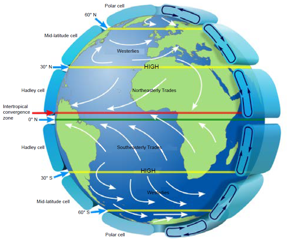
Fig. 6. Schematic of the earth’s basic tropospheric circulation, often known as the Hadley circulation. https://upload.wikimedia.org/wikipedia/commons/thumb/9/9c/Earth_Global_Circulation_-_en.svg/948px-Earth_Global_Circulation_-_en.svg.png.
2. According to Dillow (1981, 283), there would have been a large poleward movement of water vapour to balance the earth’s heat budget given the much lower level of solar radiation at the poles than at the equator, and this would have resulted in a uniform canopy base temperature. He admits that this scenario seems unlikely, but cites Venus as a parallel case in point, where the temperature at the poles is the same as at the equator. However there are important differences between Venus and the earth. Venus has a very dense atmosphere consisting mainly of carbon dioxide, resulting in a surface pressure of 92 bar. It has an axial tilt of 177º, implying that its rotation is retrograde (backwards compared with its orbital motion and with most other planets) and nearly perpendicular to its orbital plane. More importantly, Venus rotates much more slowly than the earth: its “day” lasts 243.025 earth days8. This means that its atmospheric dynamics are cyclostrophic, in which centripetal acceleration is sustained by a pressure gradient; terrestrial examples are small-scale phenomena including tornadoes, dust devils and waterspouts. In contrast, earth’s synoptic-scale atmospheric dynamics are geostrophic, in which the balance is between pressure gradient and Coriolis force due to the earth’s rotation. The atmosphere of Venus is characterised by superrotation, east-to-west zonal flows of 100 ms-1 or more at 49–70 km (30–34 mi) altitude. This is 60 times faster than the rotation of the planetary surface; these winds circle the planet within 4 earth days. Mechanisms involved in producing this fast atmospheric rotation include thermal tides, Rossby waves, Kelvin waves and gravity waves (Yamamoto 2019). Hadley cells stretch from the equator to within about 30º of the poles (Garate-Lopez et al. 2013). Both polar regions are surrounded by “cold collars” at around ±60º latitudes, inside which are relatively warm polar vortices. In particular, highly variable but persistent vortices covering on average ~2,200 × 1,400 km2 (1,400 × 900 mi2) have been observed near the south pole of Venus (Garate-Lopez et al. 2013); see fig. 7. These are essentially inverted anticyclonic vortices which form as heated air from equatorial latitudes rises and spirals rapidly towards the poles, where it converges and descends. Thus the atmospheric dynamics of Venus are very different from earth’s, which undermines confidence in Dillow’s use of Venus as an analogue of his canopied pre-Flood earth. In particular, Dillow (1981, 281) asserts that the canopy in his model prohibits “major atmospheric circulation systems (global circulation)”, which is clearly not true of Venus. Furthermore, since Dillow has not attempted to model the large-scale atmospheric dynamics of his postulated pre-Flood earth, his assertion that there would have been no global circulation has no credible basis.
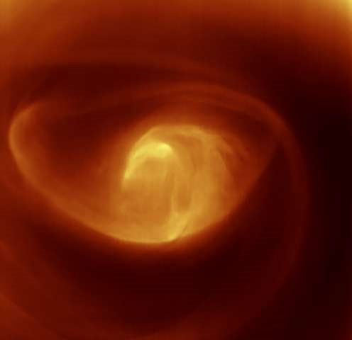
Fig. 7. Infrared image of the vortex close to the south pole of Venus, taken by the Visible and Infrared Thermal Imaging Spectrometer (VIRTIS) aboard the ESA Venus Express spacecraft. Image credit: ESA/VIRTIS/INAFISAF/ Obs. de Paris-LESIA/Univ. Oxford. The vortex is of order 2,000 km (1,200 mi) in diameter. Such vortices form because heated air from equatorial latitudes rises and spirals towards the poles, carried by fast winds. The air converges on the pole and then sinks, thereby generating a vortex. https://phys.org/news/2015-01-image-venus-snaps-swirling-vortex.html.
3. Dillow (1977; 1981, 287–304) estimates that in the presence of a vapour canopy containing 40 ft (12 m) of precipitable water, approximately 255 stars would have been visible to the naked eye at any one moment on a clear, moonless night. This is about one-tenth of the number visible today in similar conditions. Given that the sun, moon, and stars were created “to be for signs and seasons, and for days and years” (Genesis 1:14), and that God’s verdict on his completed creation was “very good” (Genesis 1:31), it is difficult to see why considerably fewer stars were visible in the primordial unspoilt creation than now, when the whole creation is suffering from the “bondage of corruption” (Romans 8:21, NKJV) and “groans and labours with birth pangs” (Romans 8:22, NKJV). The heavens, including sun, moon, and stars, serve to declare the glory of God (Psalm 19:1; 136:7–9; 147:4; 148:3) and to teach mankind humility (Psalm 8:3–4). Thus it seems natural to suppose that the stars were most clearly visible at the end of Creation Week, before Adam and Eve introduced sin and death into the world and brought a curse upon the earth (Genesis 3, notably vv. 17–18). Dillow’s view of the primordial night sky conflicts with these expectations.
4. Dillow estimates the total heat deposited on final collapse of his model vapour canopy to be 3.86 × 1024 calories (1.615 × 1025 joules), or 3.17 × 10¹⁰ joules per square metre of the earth’s surface; the main contribution is the latent heat of condensation of the vapour. Although he concedes that this enormous quantity of heat could not have been radiated away into space within 40 days of Flood rainfall, he suggests that in the last year before the onset of the Flood volcanic activity would have induced much of the canopy to condense into deep clouds. Thus most of the heat would have been radiated away or dumped into the oceans (away from Noah’s ark) as hot Flood rain. However he has not modelled this scenario or demonstrated that the proposed “deep clouds” would have been stable for long enough to accomplish the necessary radiative cooling.
5. Dillow’s vividly-presented narrative of the final collapse of the canopy and the onset of the Flood postulates widespread volcanic activity, leading to rapid cooling of the atmosphere and the earth’s surface and the rapid onset of a deep freeze in the areas where the mammoths lived. This, he suggests, led to the sudden demise of the mammoths, which he presumes not to have been cold-adapted. However modern evidence shows that mammoths were cold-adapted (Oard 2014), and it is now understood by creation scientists that mammoths flourished during the post-Flood Ice Age, their extinction resulting from unfavourable climate change at the end of the Ice Age, hunting by humans (Bartlett et al. 2016; Stuart 2015) and in some cases by genetic degeneration in isolated populations (Fry et al. 2020; Palkopoulou et al. 2015). Many mammoths were entombed in loess (wind-blown sediment). The preservation of their stomach contents (as in the Beresovka mammoth, which Dillow discusses at great length) is due to their stomach physiology rather than to a deep freeze (Batten et al. 2017b, 207–209; Oard 2000). The intense cold in Dillow’s scenario is supposedly due to the blocking of solar heating by volcanic dust and to adiabatic cooling of the atmosphere under depressurization as the canopy water fell to earth. However since the geological evidence places the Pleistocene Ice Age in the post-Flood period, this scenario now appears indefensible.
Dillow’s vapour canopy model has been criticized further on scientific grounds. Thus Wieland and Sarfati (2003) and Wieland (2010) argue that several of Dillow’s claims, mostly regarding high antediluvian atmospheric pressure and oxygen levels, and the idea that the canopy would have protected people against cosmic radiation, can no longer be supported. Wieland (1994) has also argued that declining human lifespans after the Flood were not due primarily to environmental factors, but rather to progressive degeneration of the human genome. This theme of genomic degeneration has been elaborated in depth more recently by geneticist John Sanford via the concept of “Genetic Entropy” (Sanford 2005; 2013). The idea that the pre-Flood world lacked seasons, latitudinal variation in climate, and storms (Dillow 1981; Whitcomb and Morris 1961) has been challenged by Wise (1992), who has drawn attention to growth rings found in fossil trees in strata from Devonian rocks and upwards in the geological record. The rings become generally larger and more distinct with increasing latitude, implying that the pre-Flood climate was strongly seasonal at high latitudes.
Other predictions of Dillow’s model (e.g. the Flood itself, volcanic ash mixed with ice, a sudden drop in polar temperatures, fewer meteorites in pre-Flood strata) can either be explained in other ways or have very uncertain observational support (e.g. a changed appearance of stars). His prediction of high atmospheric 3He levels turns out to be based on obsolete science. Following Whitcomb and Morris (1961, 375), Dillow (1981, 138,145–146) cites the work of Korff (1954), who estimates that the natural atmospheric abundance of 3He is about 20 times its equilibrium value. Korff assumes that: (1) the only source of atmospheric 3He is tritium (3H) production by cosmic bombardment of nitrogen in the upper atmosphere and its subsequent decay into 3He (see footnote 2), (2) the atmosphere is 3 billion years old, and (3) there has been negligible 3He loss from the atmosphere. Korff’s (1954) favoured solution is a warmer, damper atmosphere in the past than now such that the tritium production rate was enhanced by secondary cosmic ray neutrons interacting with the deuterium naturally present in the water. A further postulated source of 3He was via tritium production induced by protons ejected in solar flares, but this is insignificant (Craig and Lal 1961). However Clarke, Beg, and Craig (1969) subsequently reported excess 3He in the oceans (i.e. a higher 3He/4He ratio than in the atmosphere), which they interpreted as evidence of terrestrial primordial helium trapped in the mantle. This is now a well-established finding (Moreira 2013; Vardiman 1990). It is thus clear that degassing from the mantle is a major source of atmospheric 3He, which undermines the basis of Dillow’s (1981) prediction of high atmospheric levels of 3He.
However the most fundamental objection to Dillow’s (1981) vapour canopy model, raised by others as well as here, is that the temperature at the Earth’s surface would have been too high (Batten et al. 2017a, 174).
Subsequent Vapour Canopy Literature
Dillow (1983), evidently aware that the model presented in his 1981 book was at best incomplete, describes a more sophisticated vapour canopy model and deduces “reasonable” environmental conditions. In the 1983 paper he employs a 1D radiation balance model involving 50 wavelength bands and 20 atmospheric layers and assumes that the canopy is free of condensation nuclei, such that mist formation will only occur at saturation ratios of six or more. Although there are no obvious errors in the physics, the pressure has a local maximum in row three of Table 6, which is impossible in a static atmosphere in a vertical gravitational field; this may simply be a typographical error. The values of k (mass absorption coefficient), especially in the important 8–13 μm wavelength range, are very uncertain. Dillow (1983, 12) cites typical literature values of k = 0.01 –0.02 m2kg-1 for this range, but states that if “temperature corrected” the value could be about 0.001 m2kg-1. He subsequently (13) explains his basic problem thus (note that here Dillow quotes the units of k incorrectly)9:
The value of k used should be that k for the most transparent portion of the atmospheric infrared absorption spectrum. The value is of the order of 0.01 kg m-2 to 0.001 kg m-2 (sic) or smaller for water vapor. In the previous study, that value was applied only to the 8 to 13 micron region of the spectrum but a correct use of the Emden approximation for a dense atmosphere requires that it be applied for the terrestrial spectrum as a whole.
The results presented in Dillow’s (1983) Table 6 for vertical pressure and temperature profiles at the equator are based on the value k = 10-5m2kg-1, which is well below the experimentally supported range. He also notes that for large amounts of precipitable water in the canopy, the optical path is proportional to the square root of its precipitable water content, which implies that in the Emden approximation the effective optical path is less than the equivalent depth of water. In summary, Dillow (1983) rightly regards this version of his vapour canopy model as providing only “preliminary results”; his chosen value of k looks unduly favourable by at least an order of magnitude. Whitelaw (1983) strongly criticizes the vapour canopy theory, citing only the version proposed by Whitcomb and Morris (1961): he does not refer to Joseph Dillow’s work. Whitelaw emphasizes that the proposed canopy cannot provide more than an insignificant fraction of the vast quantity of water involved in the Flood. He also claims that the canopy theory is not supported by Scripture and that it fails against several scientific criteria. He calls his alternative the “Rift-Shift-Drift” hypothesis, which proposes that the Flood was initiated by tidal forces due to a coincidence of the earth with Mars, Ceres, and Jupiter, all at their closest approach to the sun. The tidal forces in the earth’s crust induce massive pressure waves in the magma beneath the continents, the Pacific ocean floor rises to an altitude of 5,000 ft (1.5 km) and the continents subside by 6,700 ft (2.0 km), resulting in a net rise of static sea level by 9,500 ft (2.9 km), while numerous volcanoes erupt on the Pacific floor. Whitelaw identifies these eruptions with the “fountains of the great deep” of Genesis 7:11. These, together with similar eruptions on the Indian and newly-forming Atlantic ocean floors, fill the stratosphere with steam and dust, giving rise to heavy Flood rain which continues for 40 days. Rapid continental drift and a “flip” of the earth’s rotation are also part of the picture.
In Whitelaw’s Flood scenario most of the floodwaters result from ocean water moving over continental scales in response to the vertical tectonics. Although his model is insufficiently elaborated for quantitative analysis, some of Whitelaw’s proposals have been incorporated into the Catastrophic Plate Tectonics approach to earth history (Austin et al. 1994; Baumgardner 1986), including continental-scale vertical tectonics, extensive ocean-floor volcanism and rapid continental drift. Other features are scientifically questionable: for example, the origin of the Asteroid Belt in Whitelaw’s postulated collision between Ceres and Mars conflicts with modern observations which imply the existence of several asteroid families resulting from collision-induced fragmentation of several original large bodies (Dermott et al. 2018). Several elements of Whitelaw’s scenario, notably the extraterrestrial forces invoked to trigger the Flood, are drawn from catastrophist Immanuel Velikovsky’s (1950) famously controversial Worlds in Collision and the related Earth in Upheaval (Velikovsky 1955). Jorgensen (1990; 1992; 1994—see below), in building his vapour canopy model, employs some of Whitelaw’s (1983) ideas, and consequently Velikovsky’s ideas too, though these dependencies are only acknowledged in Jorgensen (1994).
Vardiman (1986), who attempts to extend Dillow’s (1981) modelling by specially considering pre-Flood climatic conditions, was clearly influenced by Vail (1905; 1912), writing of the canopy as probably existing in four phases, i.e. as liquid droplets, ice particles, vapour and as ionized molecules. He says (114):
It is my conclusion that God probably placed the water above the firmament in all four phases. I tend to believe that the majority of the water was in the solid phase in rings surrounding the earth, but that the orbits of these rings were slowly decaying. Water was probably being slowly fed to the ionized regions and to a vapor canopy in immediate contact with the lower atmosphere. Some thin cloudiness probably occurred seasonally and diurnally.
Rush (1990) and Rush and Vardiman (1990) analyse an atmosphere containing a high-altitude water vapour canopy in radiative equilibrium. They claim (Rush and Vardiman 1990, 3) to have overcome “the lack of a sophisticated radiance program with detailed spectral data” in Dillow’s (1983) most recent paper. They ignore the effects of clouds and of convective motion. They postulate two basic requirements for acceptable pre-Flood conditions in the presence of such a canopy, viz. (1) stability of the canopy against condensation over a long period of time, and (2) a surface temperature hospitable to human beings and other life. Their results show that a canopy of between 10 mb and 1013 mb (i.e. contributing between 1% and 100% of today’s normal atmospheric pressure) would be stable in this sense, although in all cases ice particles would form at the top of the canopy (the coldest part) to produce cirrus clouds. However surface temperatures would be too high for life as we know it, certainly for a canopy of more than 50 mb. For a 50 mb canopy the calculated surface temperature is 409 K (136°C). As in Dillow’s clear-sky model, the heat problem in this case arises because of a very strong greenhouse effect due to absorption by water vapour of infrared radiation from the ground; Rush (1990) and Rush and Vardiman (1990) note how much more strongly infrared radiation is absorbed by water vapour than by carbon dioxide.
Walters (1991) seeks to address the problem of the energy load on the atmosphere arising from collapse of a Dillow-type canopy. She assumes the radiative balance conditions calculated by Rush (1990), the most sophisticated model to date of the pre-Flood atmosphere in the presence of a vapour canopy. She concludes from the energy balance that the maximum precipitable water that could be held would be about 2 ft (0.6 m), but admits the inconsistency in assuming “reasonable” temperature conditions on the basis of the Rush (1990) analysis, where the atmosphere under the canopy is hot. She treats oceans and atmosphere as lumped elements and assumes high wind speeds (averaging up to 50 mph) in order to obtain efficient heat transfer between them. The temperature rise due to canopy collapse of 50ºF from 60ºF to 110ºF (= 43.3ºC) is treated as acceptable if not comfortable; however, as already noted, the assumed initial temperature is 120ºC lower than in Rush’s (1990) model—a major inconsistency! Although various suggestions for further work are made by Walters (1991), it seems that no-one has subsequently sought to pursue this line of research, perhaps because canopy models now seem to have little currency in creationist thinking.
Jorgensen (1990; 1992) presents his own model of the pre-Flood atmosphere based on a high-altitude vapour canopy. Like Dillow, Jorgensen assumes that the earth’s pre-Flood axial tilt was close to zero. To address the question of how the earth attained its present axial tilt of almost 23½°, Jorgensen proposes an impact by a large meteor, which he suggests could also have triggered the “breakup of the oceanic lithosphere” as required by Baumgardner (1990) and induced magnetic field reversals during the Flood as proposed by Humphreys (1990); he also mentions the idea of a “large body passing close by the earth” (Jorgensen 1992, 41). One important reason for Jorgensen’s assumption of near-zero axial tilt is stated thus: “Symmetry would be achieved to give the stable atmosphere required to keep the canopy from mixing and precipitating out” (Jorgensen 1992, 41). However zero tilt only rules out seasonal changes in atmospheric conditions: it does not guarantee symmetry in longitude or about the equatorial plane, since the pre-Flood distribution of land and sea is unknown and is not considered by Jorgensen.
Contrary to Whitcomb and Morris (1961), Dillow (1981) and others, the polar regions in Jorgensen’s model are cold at the surface (-30ºC or lower), which he believes answers the question of the origin of cold-adapted animals. Accordingly his portrayal of global tropospheric wind patterns (Jorgensen 1992, Figures 6 and 7, 42) is very similar to today’s picture (fig. 6, this paper). Jorgensen proposes a very small quantity of water in the canopy, suggesting that the Flood was triggered by the break-up of the fountains of the great deep (Genesis 7:11), interpreted as volcanic activity which threw hot volcanic gases upwards into a supersaturated vapour canopy, thus causing the vapour to condense and precipitate out to produce 40 days and nights of Flood rain (Genesis 7:12).
Jorgensen (1994) attempts to systematise key elements of his model of the pre-Flood world by considering canopy conditions, possible changes in the orbits of the earth and moon, the earth’s axial tilt, “multiple ices ages” and “geological history” (287), claiming that all his proposals are supported by Scripture. He says (287):
That the Scriptures teach of a pre-Flood water Canopy has been agreed upon by many creationists for some time.
This is another example of almost equating the canopy concept with the teaching of Scripture itself. Jorgensen gives his own interpretation of Genesis 1 and 2 and proposes that the moon originally orbited the earth exactly 13 times per year of exactly 360 days until these motions were disturbed by the close passage of planetary-sized bodies. As biblically-recorded signs of these disturbances he cites various passages including Joshua 10:11–12 (the fall of massive stones from heaven and Joshua’s long day); 2 Kings 20:9–11; Isaiah 38:8 (the backward motion of the sundial shadow at the time of Hezekiah); Amos 5:8, 8:9–10; Isaiah 24:1; Job 9:6, and the Gospel accounts of the 3-hour darkness which fell during the crucifixion of Jesus. Several elements in Jorgensen’s (1994) Flood model including planetary encounters, the flipping of earth’s rotation, the rapid development of polar ice caps and changes in the length of the year and the lunar month, are based on the model outlined by Whitelaw (1983), who, as already noted, gleaned several such ideas from Velikovsky (1950; 1955).
Jorgensen (1994) suggests that the 5º inclination of the moon’s orbit from the earth’s equatorial plane may imply that the earth’s original axial tilt was 5º. He argues that evidence in Precambrian rocks conventionally understood as indicating multiple ice ages (e.g., glacial diamicts, fossils of low-temperature organisms, glacial erosional forms, glacial rhythmites, dropstones etc.) can be understood in terms of a single pre-Flood ice age, contrary to the more usual creationist view articulated by Molén (1990), who interprets this evidence in terms of gravity flows; see also Batten et al. (2017b, 199–201). Jorgensen (1994) also proposes that the earth has undergone one or more “geographic pole shifts” induced by the passage of a planetary-sized body close to the earth; he suggests that one such event caused the canopy to collapse and the earth’s magnetic field to reverse direction as seen by an earth-based observer. In these postulated events the earth’s angular momentum vector stays practically constant as seen from space, while an observer on its surface would see the sun rising in the west and setting in the east as a result of the earth rapidly “flipping over”. He claims that this would require only a relatively small input of energy, citing a paper by Warlow (1978), who refers to the analogy of a “tippe top”, a toy spinning top which naturally flips over as a result of friction while continuing to spin in the same sense. However Warlow’s dynamical analysis was criticised by Slabinski (1981), whose analysis was criticised in turn by Salkeld (1989). Whatever the truth of this argument, Jorgensen’s work has not been followed up by later creationist authors. Given Jorgensen’s assumptions, his model predicts plausible surface temperatures and plausible atmospheric temperature profiles, just as the models of Rush (1990) and Rush and Vardiman (1990) do for extremely lightweight canopies. However, the water content of his proposed canopy is far too small to contribute significantly to the enormous quantity of water involved in the Flood, and there is insufficient quantitative detail in his papers to evaluate the reliability of his results. We also note with interest the influence in Jorgensen’s thinking of catastrophist ideas gleaned from Velikovsky, i.e. from outside faithful biblical scholarship. Such an approach carries the potential danger of introducing unwarranted bias into the author’s hermeneutics.
Vardiman and Bousselot (1998) investigate the effect of varying several input parameters in models of the temperature profile under a vapour canopy, viz. solar constant (the level of solar radiation reaching the earth’s surface), albedo, solar zenith angle, cirrus cloud thickness, and cirrus cloud base height. Variations in the solar constant have the largest effect: a 50% reduction causes the computed surface temperature for a 10 mb canopy to fall from 335 K to 240 K. If all five of the above parameters are altered to give the minimum possible surface temperature, Vardiman and Bousselot estimate that the water content of the canopy could be raised to a maximum of 100 mb, or 1.0m (40in), only about 8% of that suggested by Dillow (1981)—an insignificant contribution to the Genesis Flood.
Vardiman (2003), after briefly reviewing the history of vapour canopy models, performs a series of model calculations exploring the effect of low values of the solar constant, right down to 1% of its present-day level. He shows that for a solar constant of 25% of the current value, a thick water vapour canopy would have kept the surface temperature at a liveable level. Although Vardiman is of the opinion that the solar constant could have been much lower in the past than now, he offers no evidence for this. Creationist arguments regarding the long-age uniformitarian problem known as the “Faint Young Sun Paradox” imply that solar radiation in the past was generally close to present levels (e.g., Faulkner 2001, Oard 2011, Spencer 2012; Feulner 2012 reviews the problem from a uniformitarian perspective), a position that conflicts with Vardiman’s appraisal of his modelling results. Another problem not addressed by Vardiman (2003) is the question of how the spectrum of radiation at the earth’s surface affects life. Thus if pre-Flood temperatures, despite weaker incoming solar radiation, were kept at levels similar to today’s by a strong greenhouse effect due to a vapour canopy (assisted by higher carbon dioxide levels), there would have been less visible radiation reaching the earth and proportionately more infrared radiation than we see today. The effective temperature of the solar surface today is 5772 K (Williams 2018a), and the wavelength peak in its equivalent blackbody spectrum is at 0.502 μm. The impact of a range of reduced levels of solar radiation, assumed to be due solely to a lower surface temperature, is shown in Table 1 in terms of the amount of visible light reaching the earth: note that visible radiation is critical for the process of photosynthesis on which living creatures depend, either directly or indirectly (Wikipedia 2019), and geological evidence implies a warm, wet and green (biologically productive) pre-Flood world (Humphreys 2009). Furthermore, how would humans, whose vision is limited to visible wavelengths, have fared in a world characterised by much less visible light and proportionately more infrared light than we experience today? Other possibilities cited by Vardiman (2003) for producing a reduced solar constant in the past are: (i) increased sun-earth distance, (ii) capture of radiation between sun and earth, and (iii) increased reflection from the earth’s atmosphere. However he offers no evidence in support of any of these seemingly improbable suggestions. It is thus difficult to reconcile Vardiman’s idea of a lower pre-Flood solar constant with the available evidence.
| Solar constant (percent today’s value) | Solar surface temperature Teff (K) | Wavelength peak (μm) | Infrared radiation (as fraction of total) | Total visible light (percent today’s value) |
|---|---|---|---|---|
| 100 | 5772 | 0.502 | 0.512 | 100 |
| 50 | 4854 | 0.597 | 0.639 | 41.4 |
| 25 | 4081 | 0.710 | 0.756 | 15.1 |
| 10 | 3246 | 0.893 | 0.885 | 3.01 |
| 5 | 2729 | 1.062 | 0.946 | 0.72 |
| 2 | 2171 | 1.335 | 0.985 | 0.08 |
| 1 | 1825 | 1.588 | 0.996 | 0.01 |
With the exception of Walters (1991) as discussed above, none of the vapour canopy models published since Dillow (1981) considers the final disappearance of the canopy and the related problem of the large heat load due to condensation of the vapour at the onset of the Flood. Earth’s current hydrosphere contains the equivalent of about 3.2 km (2.0 mi) depth of water over the entire surface of the planet. Therefore the canopies proposed in these models, which would deposit only 40 ft (12 m) or less of precipitable water, would have very little long-term environmental impact; there is only a problem if the heat has to be deposited quickly. Brown (2008) makes a very crude estimate of the resulting adiabatic (“immediate”) temperature rise of water and atmosphere for a canopy depositing 40 ft (12 m) of condensed water as in Dillow’s model. His answer, based on the latent heat released in condensation, is 450°C. This is patently absurd, since vapour normally only condenses in response to cooling, the release of its latent heat tending, by Le Châtelier’s principle, to counteract the cooling10, but not heating anything above its own initial temperature. The real point of Brown’s criticism is the requirement to lose heat rapidly; practically the only way the canopy can lose its heat is by radiation, and for a substantial canopy this would not occur overnight. Consider, for example, a canopy with a cloud layer beneath, the temperature of the cloud tops being 0°C; in the absence of any heat input the characteristic time for the clouds to lose all the latent heat of the vapour by blackbody radiation into space is well over two years11. As noted earlier, Dillow (1981) postulates a thick cloud layer forming in the last year before the Flood, thus providing sufficient time for the canopy to condense and radiate away much of its heat before it finally collapses. However, he has not attempted to model this, and Walters (1991, 122) regards the idea as a “weak hypothesis”.
To the knowledge of this author, there has been no attempt to model conditions on the pre-Flood earth in terms of a high-altitude vapour canopy since that of Vardiman (2003). It is also noticeable that over time, from Dillow (1981) onwards, estimates of the amount of water in the canopy declined with the increasing sophistication of the models. These observations suggest that there is little or no remaining confidence in the viability of vapour canopy models in today’s creationist community.
Conclusions
1. The idea of a high-altitude vapour canopy surrounding the pre-Flood earth did not arise within faithful mainstream biblical scholarship during the first 1,900 years of Christian history. On currently available evidence it seems to have been introduced by the long-age catastrophist Isaac Newton Vail, who attributed the idea to German Enlightenment philosopher Immanuel Kant. Whitcomb and Morris (1961) in their influential book “The Genesis Flood”, which strongly espouses the vapour canopy concept, refer to Rehwinkel (1951), who mentions it briefly; however the origin of Rehwinkel’s awareness of the idea has so far proved elusive.
2. The vapour canopy concept was developed into computationally tractable models of the earth’s pre-Flood atmosphere by several creation scientists between the 1970s and 1990s, notably by Dillow (1981; 1983), Rush (1990), Rush and Vardiman (1990), Vardiman and Bousselot (1998), and Vardiman (2003). In certain instances these authors tend towards identifying the concept with the teaching of Scripture itself, an unjustified hermeneutical approach. Whilst acknowledging that the vapour canopy concept is not directly taught in Scripture, Dillow (1981) in particular argues strongly for its superiority over alternative interpretations of the relevant passages (especially Genesis 1:6–8, 2:5–6, and 9:8–17; Psalm 148:1–6; and 2 Peter 3:5–6). However his arguments are not compelling and he has been unable to claim the general support of other interpreters.
3. All serious attempts at modelling the earth’s pre-Flood atmosphere in terms of a high-altitude vapour canopy proposed as the source of a proportion of the floodwaters either (i) predict impossibly high surface temperatures prior to the Flood, (ii) are restricted to a very thin canopy containing a trivially small amount of water, much less than originally envisaged, or (iii) invoke extremely contrived and unlikely conditions (e.g., an extremely low solar constant). The most fully articulated model (Dillow 1981) suffers from several scientific problems as well as predicting impossibly high temperatures for the pre-Flood earth. Subsequent scientific findings have not provided support for such models. While further modelling may at some future time be justified, at present a defensible, biblically and scientifically coherent vapour canopy model seems very remote. Unless a significantly better approach becomes apparent, there is no obvious reason to invest further research effort into such models except possibly to establish more completely the history of the vapour canopy concept in creationism.
Acknowledgements
Paul Garner (Biblical Creation Trust, UK) provided several of the references (books and papers) cited in this article. Kurt Wise (Truett McConnell University, Georgia, USA) advised on specific details of the contribution (or rather, non-contribution) of George McCready Price to vapour canopy models developed by creation scientists from Whitcomb and Morris (1961) onwards. Mary Smith (ICR Academic Coordinator and Registrar) provided copies of the 1990 M.S. thesis by David Rush, and Walt Stumper (AiG Educational Content Librarian) provided copies of the Whitelaw (1983) and Kaiser (2013) papers. All these forms of assistance are acknowledged with thanks.
References
Abaqus. 2017. “Mesh Convergence.” User Guide for Finite-Element Structural Analysis Software ABAQUS. https://abaqus-docs.mit.edu/2017/English/SIMACAEGSARefMap/simagsa-c-ctmmeshconverg.htm.
ACS. 2019. “A Single-Layer Atmosphere Model.” ACS (American Chemical Society) Climate Science Toolkit— How Atmospheric Warming Works. https://www.acs.org/content/acs/en/climatescience/atmosphericwarming/singlelayermodel.html.
Austin, Steven A., John R. Baumgardner, D. Russell Humphreys, Andrew A. Snelling, Larry Vardiman, and Kurt P. Wise. 1994. “Catastrophic Plate Tectonics: A Global Flood Model of Earth History.” In Proceedings of the Third International Conference on Creationism. Edited by. R. E. Walsh, 609–621. Pittsburgh, Pennsylvania: Creation Science Fellowship.
BAA. 2019. “Astronomical and Physical Constants.” In The Handbook of the British Astronomical Association 2020. Edited by Steve Harvey, 114. London, United Kingdom: British Astronomical Association, London.
Barrick, William D. 2008. “Noah’s Flood and Its Geological Implications.” In Coming to Grips with Genesis: Biblical Authority and the Age of the Earth. Edited by Terry Mortenson, and Thane H. Ury, 251–281. Green Forest, Arkansas: Master Books.
Bartlett, Lewis J., David R. Williams, Graham W. Prescott, Andrew Balmford, Rhys E. Green, Anders Eriksson, Paul J. Valdes, Joy S. Singarayer, and Andrea Manica. 2016. “Robustness Despite Uncertainty: Regional Climate Data Reveal the Dominant Role of Humans in Explaining Global Extinctions of Late Quaternary Megafauna.” Ecography 39, no. 2 (February):152–161.
Batten, Don, David Catchpoole, Jonathan Sarfati, and Carl Wieland. 2017a. “Noah’s Flood—What About All That Water?” In The Creation Answers Book, 169–178. 7th ed. Eight Mile Plains, Queensland: Creation Book Publishers.
Batten, Don, David Catchpoole, Jonathan Sarfati, and Carl Wieland. 2017b. “What About the Ice Ages? In The Creation Answers Book, 199–210. 7th ed. Eight Mile Plains, Queensland: Creation Book Publishers.
Baumgardner, John R. 1986. “Numerical Simulation of the Large-Scale Tectonic Changes Accompanying the Flood.” In Proceedings of the First International Conference on Creationism. Edited by R. E. Walsh, C. L. Brooks, and R. S. Crowell, 17–28. Pittsburgh, Pennsylvania: Creation Science Fellowship.
Baumgardner, John R. 1990. “3-D Finite Element Simulation of the Global Tectonic Changes Accompanying Noah’s Flood.” In Proceedings of the Second International Conference on Creationism. Edited by R. E. Walsh, and C. L. Brooks, 35–44. Pittsburgh, Pennsylvania, Pennsylvania: Creation Science Fellowship.
Benson, Joseph. 1857. Commentary of the Old and New Testaments. New York, New York: T. Carlton and L. Porter, New York. https://biblehub.com/commentaries/benson/.
Bixler, R. 1986. “Does the Bible Speak of a Vapor Canopy?” In Proceedings of the First International Conference on Creationism. Edited by R. E. Walsh, C. L. Brooks, and R. S. Crowell, 19–21. Pittsburgh, Pennsylvania: Creation Science Fellowship.
Brown, Walt. 2008. “Did a Water Canopy Surround the Earth and Contribute to the Flood?” In In the Beginning: Compelling Evidence for Creation and the Flood, 496. 8th ed. Phoenix, Arizona: Center for Scientific Creation.
Chandrasekhar, S. 1960. Radiative Transfer. New York, New York: Dover Publications.
Chandrasekhar, S. 1961. Hydrodynamic and Hydromagnetic Stability. New York, New York: Dover Publications..
Calvin, John. 1554. Commentary on Genesis, Volume 1 Translated by Thomas Tymme. Grand Rapids, Michigan: Christian Classics Ethereal Library. http://www.ccel.org/ccel/calvin/calcom01.
Calvin, John. 1557. Commentary on Psalms. Vol. 5. https://biblehub.com/commentaries/calvin/psalms/148.htm.
Clarke, W. B., M. A. Beg and Harmon Craig. 1969. “Excess 3He in the Sea: Evidence for Terrestrial Primordial Helium.” Earth and Planetary Science Letters 6, no. 3 (June): 213–220.
Connerney, Jack. 2013. “Saturn’s Ring Rain.” Nature 496, no. 7444 (April 11): 178–179.
Craig, Harmon, and Devendra Lal. 1961. “The Production Rate of Natural Tritium.” Tellus 13, no. 1 (February): 85–105.
Dermott, Stanley F., Apostolos A. Christou, Dan Li, Thomas J. J. Kehoe, and J. Malcolm Robinson. 2018. “The Common Origin of Family and Non-Family Asteroids.” Nature Astronomy 2, no. 7 (2 July): 549–554.
Dillow, Jody. 1977. “The Attenuation of Visible Radiation in the Vapor Canopy.” Creation Research Society Quarterly 14, no. 3 (December): 139–146.
Dillow, Joseph C. 1978a. “The Canopy and Ancient Longevity.” Creation Research Society Quarterly 15, no. 1 (June): 27–34.
Dillow, Joseph C. 1978b. “Mechanics and Thermodynamics of the Pre-Flood Vapor Canopy.” Creation Research Society Quarterly 15, no. 3 (December): 148–159.
Dillow, Joseph C. 1979. “Scripture Does Not Rule Out a Vapor Canopy.” Creation Research Society Quarterly 16, no. 3 (December): 171–173, 175.
Dillow, Joseph C. 1981. The Waters Above: Earth’s Pre-Flood Vapour Canopy. Chicago, Illinois: Moody Press.
Dillow, Joseph C. 1983. “The Vertical Temperature Structure of the Pre-Flood Vapor Canopy.” Creation Research Society Quarterly 20, no. 1 (June): 7–14.
Faulkner, Danny. 2001. “The Young Faint Sun Paradox and the Age of the Solar System.” TJ 15, no. 2 (August): 3–4.
Faulkner, Danny R. 2016. “Thoughts on the rāqîa‘ and a Possible Explanation for the Cosmic Microwave Background.” Answers Research Journal 9 (March 23): 57–65.
Faulkner, Danny R. 2018. “The Current State of Creation Astronomy II.” In Proceedings of the Eighth International Conference on Creationism. Edited by J. H. Whitmore, 36–45. Pittsburgh, Pennsylvania: Creation Science Fellowship.
Feulner, Georg. 2012. “The Faint Young Sun Problem.” Reviews of Geophysics 50, no. 2 (June): RG2006. 29 pages. doi: 10.1029/2011RG000375.
Fouts, David M. 2015. Right from the Start! Calling Evangelical Leadership to Faith in Genesis 1–2. Amazon Services: self-published.
Frazer, Sir James George. 1918. Folklore in the Old Testament. Vol. 1. London, United Kingdom: Macmillan.
Fry, Erin, Sun K. Kim, Sravanthi Chigurapti, Katelyn M. Mika, Aakrosh Ratan, Alexander Dammermann, Brian J. Mitchell, Webb Miller, and Vincent J. Lynch. 2020. “Functional Architecture of Deleterious Genetic Variants in the Genome of a Wrangel Island Mammoth.” Genome Biology and Evolution 12, no. 3 (March): 48–58.
Garate-Lopez, I., R. Hueso, A. Sánchez-Lavega, J. Peralta, G. Piccioni, and P. Drossart. 2013. “A Chaotic Long-Lived Vortex at the Southern Pole of Venus.” Nature Geoscience 6, no. 4 (March): 254–257.
Gargallo-Peiró, Abel, Matias Avila, Herbert Owen, Luis Prieto-Godino, and Arnau Folch. 2018. “Mesh Generation, Sizing and Convergence for Onshore and Offshore Wind Farm Atmospheric Boundary Layer Flow Simulation with Actuator Discs.” Journal of Computational Physics 375 (15 December): 209–227.
Gebhart, B. 1971. Heat Transfer. 2nd ed. Texas, USA: McGraw-Hill.
Gill, John. 1746–1763. Exposition of the Entire Bible. https://www.sacred-texts.com/bib/cmt/gill/gen001.htm.
Goode, P. R., J. Qiu, V. Yurchyshyn, J. Hickey, M.-C. Chu, E. Kolbe, C. T. Brown, and S. E. Koonin. 2001. “Earthshine Observations of the Earth’s Reflectance.” Geophysical Research Letters 28, no. 9 (1 May): 1671–1674.
Hartnett, J. 2007. Starlight, Time and the New Physics. Eight Mile Plains, Queensland: Creation Book Publishers.
Hebert, Jake. 2017. “Have Creationists Overlooked an Abundance of Biblical Cosmological Data?” Creation Research Society Quarterly 5, no. 4 (Spring): 286–296.
Henry, Matthew. 1706. Commentary on the Whole Bible. Vol. 1. Genesis to Deuteronomy. Grand Rapids, Michigan: Christian Classics Ethereal Library. http://www.ccel.org/ccel/henry/mhc1.pdf.
Hodge, Bodie. 2019. “What Is the State of the Water Vapor Canopy Model?” In “The New Answers Book 4”. Edited by Ken Ham and Bodie Hodge. Green Forest, Arkansas: Master Books.
Holton, James R. 2004. An Introduction to Dynamic Meteorology. 4th ed. Amsterdam, Netherlands: Elsevier.
Humphreys, D. Russell. 1978. “Is The Earth’s Core Water? Part One: The Biblical Evidence.” Creation Research Society Quarterly 15, no. 3 (December): 141–147.
Humphreys, D. Russell. 1990. “Physical Mechanisms for Reversals of the Earth’s Magnetic Field During the Flood.” In Proceedings of the Second International Conference on Creationism. Edited by R. E. Walsh and C. L. Brooks, 129–140. Pittsburgh, Pennsylvania: Creation Science Fellowship.
Humphreys, D. Russell. 1994a. “A Biblical Basis for Creationist Cosmology.” In Proceedings of the Third International Conference on Creationism. Edited by R. E. Walsh, 255–266. Pittsburgh, Pennsylvania: Creation Science Fellowship.
Humphreys, D. Russell. 1994b. “Starlight and Time.” Green Forest, Arkansas: Master Books.
Humphreys, D. Russell. 2007. “Creationist Cosmologies Explain the Anomalous Acceleration of the Pioneer Spacecraft.” Journal of Creation 21, no. 2 (August): 61–70.
Humphreys, Russ. 2009. “God’s Global Warming Worked Just Fine: Evidence From the pre-Flood World Suggests That We Need Not Fear Global Warming From Carbon Dioxide.” Viewpoint, 11 August. Creation Ministries International. https://creation.com/global-warming-facts-and-myths.
Johnson, Gary L. 1987. “The Firmament: A Hypothesis.” Creation Research Society Quarterly 24, no. 1 (June): 38–42.
Jorgensen, G. S. 1990. “A Computer Model of the Pre-Flood Atmosphere.” In Proceedings of the Second International Conference on Creationism. Edited by R. E. Walsh, and C. L. Brooks, 143–149. Pittsburgh, Pennsylvania: Creation Science Fellowship.
Jorgensen, G. S. 1992. “Fundamental Physics of a Water Vapor Canopy Atmosphere.” In Proceedings of the 1992 Twin-Cities Creation Conference, 40–45. Minneapolis, Minnesota: Twin-Cities Creation Science Association.
Jorgensen, Greg S. 1994. “The Canopy, the Moon, the Tilt of the Earth’s Axis, and a Pre-Flood Ice Age.” In Proceedings of the Third International Conference on Creationism. Edited by R. E. Walsh, 287–303. Pittsburgh, Pennsylvania: Creation Science Fellowship.
Kaiser, Walter C. Jr. 2013. “A Literal and Historical Adam and Eve? Reflections on the Work of Peter Enns.” Criswell Theological Review 10, no. 2 (Spring): 75–82.
Kant, Immanuel. 1755 (2012). Universal Natural History and Theory of the Heavens. users.clas.ufl.edu/burt/spaceshotsairheads/Kantuniversalnaturalhistory.pdf.
Keil, C. F., and F. Delitzsch. 1869. Biblical Commentary on the Old Testament. Vol. 1. The Pentateuch. Translated by Rev. James Martin. Edinburgh, United Kingdom: T. and T. Clark. https://biblehub.com/commentaries/kad/genesis/1.htm.
Keil, C. F. and F. Delitzsch. 1871 Biblical Commentary on the Old Testament. Vol. 5. Psalms. Translated by Francis Bolton. https://biblehub.com/commentaries/kad/psalms/148.htm.
Kidner, Derek. 1976. Genesis: An Introduction and Commentary. Leicester, England: Inter-Varsity Press.
Kofahl, Robert E. 1977. “Could the Flood Waters Have Come From a Canopy or Extraterrestrial Source?” Creation Research Society Quarterly 13, no. 4 (March): 202–206.
Korff, Serge A. 1954. “Effects of the Cosmic Radiation on Terrestrial Isotope Distribution.” EOS, Transactions, American Geophysical Union 35, no. 1 (February): 103–106.
Leupold, H. C. 1942. Exposition of Genesis. Columbus, Ohio: The Wartburg Press.
Lisle, J. 2019. “No Rain?” https://biblicalscienceinstitute.com/apologetics/no-rain/.
Lucas, Dick, and Christopher Green. 1995. The Message of 2 Peter and Jude. The Bible Speaks Today. Leicester, United Kingdom: Inter-Varsity Press.
Ludlam, F. H., and R. S. Scorer. 1960. Cloud Study: A Pictorial Guide. London, United Kingdom: John Murray.
Luther, Martin. 1544a (1904). Commentary on Genesis. Vol. 1. Luther on the Creation. Edited by John Nicholas Lenker. Minneapolis, Minnesota: Lutherans in All Lands Co.
Luther, Martin. 1544b (1910). Commentary on Genesis. Vol. 2. Luther on Sin and the Flood. Edited by John Nicholas Lenker. Minneapolis, Minnesota: The Luther Press.
McCabe, Robert V. 2008. “A Critique of the Framework Interpretation of the Creation Week.” In Coming to Grips with Genesis: Biblical Authority and the Age of the Earth. Edited by Terry Mortenson, and Thane H. Ury, 211–249. Green Forest, Arkansas: Master Books.
McIver, Tom. 1988. Anti-Evolution: An Annotated Bibliography. Jefferson, North Carolina: McFarland and Company.
Met Office. 2020. “Global Circulation Patterns” https://www.metoffice.gov.uk/weather/learn-about/weather/atmosphere/global-circulation-patterns.
Migne, J.-P. 1845. Patrologia Latina 22:659. https://books.google.co.uk/books?id=CUkwAAAAYAAJ&pg=RA4-PT204&source=gbs_toc_r&cad=4#v=onepage&q&f=true.
Molén, Mats. 1990. “Diamictites: Ice-Ages or Gravity Flows?” In Proceedings of the Second International Conference on Creationism. Edited by R. E. Walsh, and C. L. Brooks, 177–190. Pittsburgh, Pennsylvania: Creation Science Fellowship.
Moreira, Manuel. 2013. “Helium Isotopes and the Two-Reservoir Mantle Story.” Geochemical Perspectives 2, no. 2 (July): 267–282.
Morton, Glenn R. 1979. “Can the Canopy Hold Water?” Creation Research Society Quarterly 16, no. 3 (December): 164–169.
Morton, Glenn R. 1980. “Objections to an Ice Canopy.” Creation Research Society Quarterly 17, no. 2 (September): 138.
Morton, Glenn R. 1982. “Comments on The Waters Above.” Creation Research Society Quarterly 19, no. 1 (June): 78–80.
Oard, Michael. 2000. “The Extinction of the Woolly Mammoth: Was it a Quick Freeze?” Creation Ex Nihilo Technical Journal 14, no. 3 (December): 24–34.
Oard, Michael J. 2011. “Is the Faint Young Sun Paradox Solved?” Journal of Creation 25, no. 2 (August): 17–19.
Oard, Michael. 2014. “Woolly Mammoths Were Cold Adapted.” Journal of Creation 28, no. 3 (December): 15–17.
O’Donoghue, J., T. S. Stallard, H. Melin, G. H. Jones, S. W. H. Cowley, S. Miller, K. H. Baines, and J. S. D. Blake. 2013. “The Domination of Saturn’s Low-Latitude Ionosphere by Ring ‘Rain’.” Nature 496, no. 7444 (11 April): 193–195.
O’Donoghue, James, Luke Moore, Jack Connerney, Henrik Mellin, Tom S. Stallard, Steve Miller and Kevin H. Baines. 2019. “Observations of the Chemical and Thermal Response of ‘Ring Rain’ on Saturn’s Ionosphere.” Icarus 322 (April): 251–260.
Palkopoulou, Eleftheria, Swapan Mallick, Pontus Skoglund, Jacob Enk, Nadin Rohland, Heng Li, Ayça Omrak, Sergey Vartanyan, Hendrik Poinar, Anders Götherström, David Reich, and Love Dalén. 2015. “Complete Genomes Reveal Signatures of Demographic and Genetic Declines in the Woolly Mammoth.” Current Biology 25, no. 10 (18 May): 1395–1400.
Poole, Matthew. 1685. A Commentary on the Holy Bible. Vol. 1. https://biblehub.com/commentaries/poole/genesis/1.htm.
Price, George McCready. 1923. The New Geology. Mountain View, California: Pacific Press Publishing Association.
Rehwinkel, Alfred M. 1951. The Flood in the Light of the Bible, Geology and Archaeology. St. Louis, Missouri: Concordia Publishing House.
Richardson, Lewis Fry. 1911. “The Approximate Arithmetical Solution by Finite Differences of Physical Problems Involving Differential Equations, with an Application to the Stresses in a Masonry Dam.” Philosophical Transactions of the Royal Society A 210, nos. 459–470 (1 January): 307–357.
Rush, D. E. 1990. Radiative Equilibrium Temperature Profiles under a Vapor Canopy. M.S. Thesis. Institute for Creation Research, El Cajon, California.
Rush, David E., and Larry Vardiman. 1990. “Pre-Flood Vapor Canopy Radiative Temperature Profiles.” In Proceedings of the Second International Conference on Creationism. Edited by R. E. Walsh, and C. L. Brooks, 231–240. Pittsburgh, Pennsylvania: Creation Science Fellowship.
Sakri, F. Mohd, M. S. Mat Ali, and S. A. Z. Sheikh Salim. 2016. “Computational Investigations and Grid Refinement Study of 3D Transient Flow in a Cylindrical Tank Using OpenFOAM.” IOP Conference Series: Materials Science and Engineering 152: 012058. doi: 10.1088/1757-899X/152/1/012058.
Salkeld, David. 1989. “Objections Overruled—A Reappraisal of Earth Inversion Dynamics.” Chronology and Catastrophism Review 11: 29–34.
Sanford, J. C. 2005. Genetic Entropy and the Mystery of the Genome. 2nd ed. Lima, New York: Elim Publishing, Lima, New York.
Sanford, John. 2013. “Critic ignores reality of Genetic Entropy.” Creation Ministries International. http://creation.com/genetic-entropy.
Sarfati, Jonathan. 2010. “Flood Models and Biblical Realism.” Journal of Creation 24, no. 3 (December): 46–53.
Schaeffer, Francis A. 1968. Escape from Reason. Downs Grove, Illinois: Inter-Varsity Press.
Slabinski, V. J. 1981. “A Dynamic Objection to the Inversion of the Earth on its Spin Axis.” Journal of Physics A: Mathematical and General 14, no. 9 (1 September): 2503–2507.
Slater, John W. 2008. “Examining Spatial (Grid) Convergence.” NPARC Alliance CFD Verification and Validation Web Site. https://www.grc.nasa.gov/WWW/wind/valid/tutorial/spatconv.html.
Spencer, Wayne. 2012. “New Science on the Young Sun, and Earth Migration.” Journal of Creation 26, no. 3 (December): 5–7.
Strickling, James E. 1976. “The Waters Above the Firmament.” Creation Research Society Quarterly 12, no. 4 (March): 221.
Strutt, John William. 1917. “On the Dynamics of Revolving Fluids.” Proceedings of the Royal Society A. 93, no. 648 (1 March): 148–154.
Stuart, Anthony John. 2015. “Late Quaternary Megafaunal Extinctions on the Continents: A Short Review.” Geological Journal 50, no. 3 (May/June): 338–363.
Taylor, Charles V. 1996. “Waters Above or Beyond?” Creation Ex Nihilo Technical Journal 10, no. 2 (August): 211–213.
Taylor, Geoffrey Ingram. 1923. “Stability of a Viscous Liquid Contained Between Two Rotating Cylinders.” Philosophical Transactions of the Royal Society A 223, nos. 605–615 (1 January): 289–343.
The Velikovsky Encyclopedia. 2019. Isaac Vail. https://www.velikovsky.info/isaac-vail/.
Udd, Stanley V. 1975. “The Canopy and Genesis 1:6–8.” Creation Research Society Quarterly 12, no. 2 (September): 90–93.
Vail, Isaac Newton. 1902. The Waters Above the Firmament, or The Earth’s Annular System. 2nd ed. Philadelphia: Ferris and Leach. https://archive.org/details/watersabovefirma00vail/page/n5.
Vail, Isaac Newton. 1905. The Deluge and its Cause. Chicago, Illinois: Suggestion Publishing Company. https://archive.org/details/delugeitscausebe00vail/page/n5.
Vail, Isaac N. 1912. The Earth’s Annular System, or The Waters Above the Firmament. 4th ed. Pasadena, California: The Annular World Company. https://babel.hathitrust.org/cgi/pt?id=uc2.ark:/13960/t8rb6x64b&view=1up&seq=5.
Vardiman, Larry. 1986. The Sky Has Fallen. In Proceedings of the First International Conference on Creationism. Edited by R. E. Walsh, C. L. Brooks, and R. S. Crowell, 113–119. Pittsburgh, Pennsylvania: Creation Science Fellowship.
Vardiman, Larry. 1990. The Age of the Earth’s Atmosphere. El Cajon, California: Institute for Creation Research.
Vardiman, Larry, and Karen Bousselot. 1998. Sensitivity Studies on Vapor Canopy Temperature Profiles. In Proceedings of the Fourth International Conference on Creationism. Edited by R. E. Walsh, 607–618. Pittsburgh, Pennsylvania: Creation Science Fellowship.
Vardiman, Larry. 2003. Temperature Profiles for an Optimized Water Vapor Canopy. In Proceedings of the Fifth International Conference on Creationism. Edted by R. L. Ivey, 29–39. Pittsburgh, Pennsylvania: Creation Science Fellowship.
Velikovsky, Immanuel. 1950. Worlds in Collision. New York, New York: Macmillan.
Velikovsky, Immanuel. 1955. Earth in Upheaval. Garden City, New York: Doubleday and Company.
Walters, Tracy W. 1991. “Thermodynamic Analysis of a Condensing Vapor Canopy.” Creation Research Society Quarterly 28, no. 3 (December): 122-131.
Warlow, P. 1978. “Geomagnetic Reversals?” Journal of Physics A: Mathematical and General 11, no. 10 (October): 2107–2130.
Westberg, V. Luther. 1979. “Floodtime Changes in the Earth’s Heating and Lighting.” Creation Research Society Quarterly 16, no. 3 (December): 182–184.
Westberg, V. Luther. 1980. “Reply to Morton.” Creation Research Society Quarterly 17, no. 2 (September): 138.
Whitcomb, John C., and Henry M. Morris. 1961. The Genesis Flood: The Biblical Record and Its Scientific Implications. Philadelphia, Pennsylvania: Presbyterian and Reformed Publishing Company.
Whitelaw, Robert L. 1983. “The Fountains of the Great Deep, and the Windows of Heaven.” In Science at the Crossroads: Observation or Speculation? 95–104. Papers of the 1983 National Creation Conference, Bible-Science Association and Twin Cities Creation Science Association. Onesimus Publishing: Richfield, Minnesota.
Wieland, Carl. 1989. “‘Hanging Loose’: What Should We Defend?” Creation 11, no. 2 (March): 4.
Wieland, Carl. 1994. “Decreased Lifespans: Have We Been Looking in the Right Place?” Creation Ex Nihilo Technical Journal 8, no. 2 (August): 138–141.
Wieland, Carl. 2010. “Blame CMI? And What About the “Canopy” Theory?” http://creation.com/cannot-blame-cmi.
Wieland, Carl, and Jonathan Sarfati. 2003. “Running Out Of Puff: Low Oxygen May Have Medical Benefits—Implications for the ‘Vapour Canopy’ Model.” http://creation.com/running-out-of-puff.
Wikipedia. 2019. “Photosynthetically Active Radiation.” http://en.wikipedia.org/wiki/Photosynthetically_active_radiation.
Williams, David R. 2018a. “Sun Fact Sheet.” http://nssdc.gsfc. nasa.gov/planetary/factsheet/sunfact.html.
Williams, David R. 2018b. “Venus Fact Sheet.” https://nssdc. gsfc.nasa.gov/planetary/factsheet/venusfact.html.
Wise, Kurt P. 1992. “Were There Really No Seasons? Tree Rings and Climate.” Creation Ex Nihilo Technical Journal 6, no. 2 (August): 168–172.
Wise, Kurt P. 2018. “Contributions to Creationism by George McCready Price.” In Proceedings of the Eighth International Conference on Creationism. Edited by J. H. Whitmore, 683–694, Pittsburgh, Pennsylvania: Creation Science Fellowship.
Wise, K. P. 2019. Personal e-mail communication, 18 November 2019.
Worraker, William. 2018. “Heat Problems Associated with Genesis Flood Models—Part 1: Introduction and Thermal Boundary Conditions.” Answers Research Journal 11 (July 11): 171–191.
Worraker, William. 2019. “Heat Problems Associated with Genesis Flood Models—Part 2: Secondary Temperature Indicators.” Answers Research Journal 12 (September 18): 211–254.
Yamamoto, Masaru. 2019. “Atmospheric Circulation on Venus.” Oxford Research Encyclopedia of Planetary Science. https://oxfordre.com/planetaryscience. doi: 10.1093/acrefore/9780190647926.013.117.
Young, Edward J. 1964. Studies in Genesis One. Grand Rapids, Michigan: Baker Book House.
Younker, Randall W., and Richard M. Davidson. 2011. “The Myth of The Solid Heavenly Dome: Another Look at the Hebrew רָקיִע (rāqîaʿ).” Andrews University Seminary Studies 49, no. 1: 125–147.
Appendix: Analysis of Joseph Dillow’s (1981) “Cloud Canopy” Model
Dillow’s (1981, 240–243) 3-layer model of the troposphere assumes grey radiation, i.e. all relevant atmospheric properties (emissivity and absorption coefficient) are wavelength-independent. Surface emissivity values are 1.0 (i.e. everything radiates as a pure blackbody), and the base temperature of the clouds is 373 K (≈100°C). Dillow allows for radiation absorption through each layer, the transmitted fraction being 0.4 in layer 1 (nearest to the clouds), 0.5 in layer 2 and 0.6 in layer 3 (nearest to the surface), corresponding to a decrease in the density of water vapour from the canopy base to the surface (Dillow 1981, 243). Dillow claims that this gives a surface temperature of 293 K or 20°C (= 68°F), though he does not say how he has obtained this figure. However his fig. 7.2 (fig. 4, this paper) gives T1 = 55°C, T2 = 39°C, and T3 = 23°C. The radiation balance equations he is solving are summarised in his equation (7.24), which in matrix form would be written (using his notation):
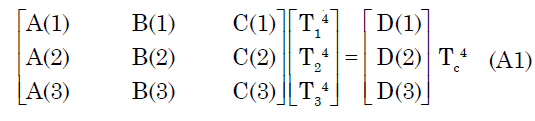
Here Tc is the cloud base temperature (given as 373 K). Since all the terms in the 3×3 frontal matrix and on the right-hand side are known, this equation can readily be solved by matrix inversion. However, radiation from the surface, although indicated in Dillow’s fig. 7.2 (fig. 4 here), is not accounted for in his equation (7.24). If the matrix entries in equation (A1) are constructed as indicated by Dillow, the resulting temperatures are T1 = 21°C, T2 = –15°C, and T3 = –52°C. Including the radiation from the surface in the balance equations produces a 4 × 4 matrix equation of the form
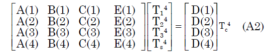
In this case, with the E() terms constructed on the same principles, the resulting temperatures are T1 = 55°C, T2 = 41°C, and T3 = 24°C, very close to those quoted by Dillow. However Ts = 100°C, equal to Tc and much higher than the figure quoted by Dillow. A further check on his results may be carried out by changing the number of atmospheric layers in the model, since this number is a free choice for the modeller and should not significantly affect the vertical temperature profile12. Such a check has been carried out by comparing the results for 2, 3, 4, 5, and 6 tropospheric layers between the clouds and the surface. To maintain comparability with Dillow, the fraction of radiation emitted from the cloud base which reaches the surface without absorption is kept at 0.12 in all cases; for more than 3 layers the individual transmitted fractions are chosen to increase from top to bottom in a geometric sequence. The equations (in matrix form) are readily solved on an ©Excel spreadsheet using the ©MINVERSE and ©MMULT functions. The results are shown in table 2. There is a clear trend here: the temperatures in the first and last layers decrease monotonically with an increasing number of layers, which does not make physical sense, especially given that the surface temperature is 100°C in all cases.
| Number of layers | Transmitted fractions | T (highest layer), °C | T (lowest layer), °C | T (surface), °C |
|---|---|---|---|---|
| 2 | 0.3, 0.4 | 68.2 | 55.3 | 100 |
| 3 | 0.4, 0.5, 0.6 | 55.3 | 23.6 | 100 |
| 4 | 0.45, 0.54, 0.64, 0.77 | 48.5 | -15.8 | 100 |
| 5 | 0.49, 0.57, 0.65, 0.75, 0.87 | 41.4 | -47.1 | 100 |
| 6 | 0.55, 0.61, 0.67, 0.74, 0.81, 0.89 | 31.8 | -58.9 | 100 |
The basic problem with Dillow’s model is that he has not taken account of the relationship between absorption and emission for individual tropospheric layers. For each layer transmissivity (α) and emissivity (ε) must be complementary (radiation not transmitted through a layer is absorbed and reemitted), as exemplified, for example, in the simple atmospheric model presented by ACS (2019). This is a consequence of Kirchhoff’s radiation law, which states that in an atmosphere characterised by negligible scattering and therefore in local thermodynamic equilibrium, a local temperature can be defined such that absorption and emission must be in balance at every wavelength and in every direction. Thus the emission at frequency ν is given by

where jν is the radiant power emitted at frequency ν per unit mass per unit solid angle per Hertz, κν is the mass absorption coefficient and the Planck function at temperature T is given by

h and k being the Planck and Boltzmann constants respectively, and c the speed of light (Chandrasekhar 1960, equations 38 and 39). This is equivalent to stating that εν + αν = 1 at any point and at any frequency ν. The integrated form of this relationship for the entire frequency range of the radiation follows from this. Thus εi = 1 –αi for each layer i in Dillow’s model such that the total radiation in each direction (up or down) is εiσTi4= (1 –αi)σTi4; the emissivity factor is missing in Dillow’s equations. If his equations are corrected accordingly, the resulting temperature is 100ºC throughout his model, regardless of the number of layers; there is no temperature inversion.
The reason for this result is fundamental: a system characterised by a single fixed temperature (the cloud base temperature Tc) and no net external heat flux and no internal heat source or sink will reach a uniform equilibrium temperature regardless of the heat transfer mechanism. Thus the surface temperature Ts and the air temperature T below the clouds must equal the only fixed temperature available, the temperature of the cloud base. This result is obtained more formally by solving the equation for 1-dimensional heat transfer in a nonopaque medium in which heat transfer is dominated by grey radiation, viz.

(Gebhart 1971, 166), where x represents distance, kR plays the role of thermal conductivity and A is a constant which is not subsequently needed. If the earth’s surface corresponds to x = 0 and the cloud base to x = L, then the relevant boundary conditions are dT/dx(0) = 0 and T(L) = Tc; the condition at x = 0 is based on zero net heat flux through the surface, implicitly in line with Dillow (1981), Morton (1979) and other atmospheric modellers. The solution is then simply T(x) = Tc, and so the surface temperature is Ts = Tc.
This result is not affected by surface emissivities of less than unity because radiation not absorbed and re-emitted will be reflected instead; for the grey approximation the troposphere cannot distinguish between reflected and reemitted radiation. Thus the troposphere and the earth’s surface will heat up to the temperature of the cloud base; the surface temperature would still have been too high for life.
Dillow (1981) goes on to propose that a model of the atmosphere capped by a cloud layer with a fixed base temperature would give more reliable results if the radiation balance were handled in terms of discrete wavelength bands. No such exercise is reported in his 1981 book, but I have undertaken a simple version of the proposed calculations by setting up 1D models including 1, 2, and 3 atmospheric layers. In these models the radiation is divided into three wavelength bands, viz U, denoting ultraviolet and shorter wavelengths, V denoting visible wavelengths (between 0.4 and 0.7 microns) and I, denoting infrared and longer wavelengths. In the present-day atmosphere most of the incoming ultraviolet solar radiation is absorbed by ozone (O3) in the stratosphere, most visible light is transmitted to the surface, and a significant fraction of the infrared and microwave radiation is absorbed by water vapour, CO2 and other greenhouse gases.
If the average solar radiation reaching the earth is denoted S0 (approximately 340.3 Wm-2) and has the spectrum corresponding to a black body at 5772 K (Williams 2018a; this is the effective surface temperature of the sun, to be denoted Teff), we denote its division into wavelength bands by the fractions fU(Teff), fV(Teff), and fI(Teff) for the U, V, and I bands respectively, where fU + fV + fI = 1. If the atmospheric layers in our models are labelled j where j = 1, n (n is the number of layers), then the emissivities for each band are labelled εjU, εjV, and εjI, and the corresponding transmissivities αjU, αjV, and αjI.
Consider a single-layer model described in terms of this formalism, with the earth’s surface denoted by s, and hence its temperature Ts. We ignore reflection and scattering and other complicating factors also ignored by Dillow (1981). The radiation balance for the single atmospheric layer is thus written
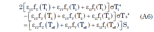
and for the surface
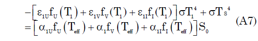
where we have taken the earth’s surface to be radiating as a black body, such that εsU = εsV = εsI = 1. The radiation fractions for the incoming solar radiation are fU(Teff) = 0.1218, fV(Teff) = 0.3665, and fI(Teff) = 0.5117, while the fractions for blackbody radiation from terrestrial sources at temperatures of 373 K or below are, for all practical purposes, fU (Ts) = 0.0, fV(Ts) = 0.0, and fI (Ts) = 1.0, and similarly for T1 etc. We take ε1U = 1.0, ε1V = 0.0, and ε1I = 0.66. Writing S0/σ = 6.00138 × 10⁹ K4, equations (A4) and (A5) may be written in matrix form as

where the 2 × 2 matrix A11 = has components A11 = 2 [ ε1U fU(T1) + ε1VfV(T1) + ε1IfI(T1) ] , A12 = –[ ε1UfU(Ts) + ε1VfV(Ts) + ε1IfI(Ts) ] , A21 = –[ε1UfU(T1) + ε1V fV(T1) + ε1IfI(T1)], and A22 = 1.0. Also X1 = T14, X2 = Ts4, B1 = ε1UfU(Teff) + ε1VfV(Teff) + ε1IfI(Teff) and B2 = α1UfU(Teff) + α1VfV(Teff) + α1IfI(Teff). With the above values inserted, the solution of equation (A8) is T1 = 272.81 K (–0.34ºC), Ts = 288.20 K (15.05ºC). Even this extremely simplified model shows how atmospheric absorption of infrared radiation warms the earth’s surface: with no atmosphere at all the earth’s surface temperature, if radiating as a pure blackbody and assuming no reflection (zero albedo), would be at an average temperature of 278.33 K (5.18ºC).
Next consider the same atmospheric model, but this time without solar heating. Instead, as per Dillow’s suggested multiwavelength model in this context, assume the atmosphere to be capped by a cloud layer with a base temperature Tc of 100ºC (373.15 K) and radiating as a black body. While the lefthand side of equation (A8) would remain the same, S0/σ on the righthand side is replaced by Tc4, and we would now have B1= ε1UfU(Tc) + ε1VfV(Tc) + ε1lfl(Tc) and B2 = α1UfU(Tc) + α1VfV(Tc) + α1IfI(Tc). The crucial difference is that all the radiation is now in the I band, such that fU (Tc) = 0, fV (Tc) = 0, and fI(Tc) = 1.0. The solution of the equivalent to (A8) is then simply T1 = Ts = Tc = 373.15 K as in the grey approximation discussed above.
A similar exercise has been carried out in an ©Excel spreadsheet for a four-band, eight-layer model of the atmosphere in which the I band as defined above is now divided into infrared or I radiation (wavelength 0.7–8.0 μm) and longwave or L radiation (wavelength greater than 8.0 μm). Values of transmitted fraction α in the I and L bands for individual layers have been chosen to ensure that the total transmitted fraction through all the layers in these bands are in the region of 0.12, individual values decreasing from top to bottom in geometric and arithmetic progressions. Transmitted fraction values in the L band are chosen close to (but not identical to) I band values. In all cases investigated a cloud-topped atmosphere gave temperatures everywhere identical to the cloud base temperature, viz. 373.15 K, as expected from first principles. The equivalent cases with cloud heating replaced by solar heating produced a variety of atmospheric temperature profiles depending on the chosen transmitted fractions.
Contrary to Dillow’s (1981) suggestion, more sophisticated versions of such a multiwavelength model must give the same result: as noted above, a system characterised by a single fixed temperature (the cloud base temperature Tc) and no net external heat flux will reach a uniform equilibrium temperature equal to Tc. The previous conclusion still applies: the surface temperature would have been too high for life. Meaningful tropospheric temperature profiles can be calculated if the cloud base temperature is left unspecified and solar heating is included in the radiation balance, but such conditions conflict with the conceptual basis of Dillow’s “cloud canopy” model.
In conclusion, this “cloud canopy” model, in both published and more sophisticated forms, does not solve the heat problem in Dillow’s (1981) vapour canopy model, even in the absence of the heavy rain it would almost certainly produce.


