
Chapter 10
Catastrophic Melting
Accelerated melting would mark the end of the Ice Age.
According to the creation-Flood Ice Age model, glacial maximum was reached when the ocean temperature cooled to an average of 50°F (10°C). At this ocean temperature, the net melting of the glaciers would be slow. Precipitation would still be substantial, but would decrease with time. As the oceans continued to cool, the amount of water evaporating into the atmosphere would continue to decrease proportionate to the ocean’s surface temperature. Accelerated melting would mark the end of the Ice Age.
Warmer Summers, Colder Winters
As the Ice Age waned, volcanism gradually decreased as the earth became used to the new configuration of land and water caused by the Flood. Less gas and ash spewed into the stratosphere, and more sunlight warmed the summers. Summers, of course, would not be as warm as they are today in the mid and high latitudes because the nearby ice sheets and increased sea ice would keep the land somewhat cool.
A decrease in volcanic activity would also affect the tropics. Temperatures there would warm quite quickly and would soon approximate today’s climate. Due to the slower melting of the ice sheets at higher latitudes, the tropical to polar temperature difference would be greater than it is today. This difference in atmospheric temperature is very important for understanding the demise of the woolly mammoth and other animals. This is because such a temperature difference would cause strong, windy, dry storms.
At the same time as the decreased volcanism, the ocean water would continue cooling and sea ice would gradually develop in the polar latitudes. These two factors would result in a drying atmosphere in this phase of the Ice Age. Sea ice would form quickly because meltwater from melting ice sheets would flow out over the ocean water at mid and high latitudes. Fresh water has a tendency to float on the denser salt water, making it easier to form ice. Sea ice, especially with fresh snow on top, would reinforce the winter cooling trend by reflecting sunlight back into space. It would also stop the heat of the warmer water from entering the atmosphere. Thus, sea ice would increase the cooling of the atmosphere, which would further increase ocean cooling, sort of like a chain reaction.
The net effect of this climatic change would be that winters would become quite cold and the summers mild as the ice sheets melted. Winters would be significantly colder than today, and summers warmer, but not as warm as today. The atmosphere would also become drier and drier. The climate over mid- and high-latitude continents would become more continental with colder winters and warmer summers. During the earlier phase when the ice was building up, the climate was equitable, having little seasonal contrast, but during deglaciation, snowfall on the ice sheets would be light and would easily melt by the time summer arrived. The winter cooling and drying would continue until the ice sheets melted. Figure 10.1 shows the generally expected temperature trend through the Ice Age to the present for the mid- and high-latitude continents of the Northern Hemisphere.
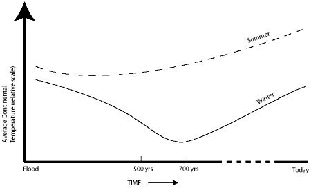
Figure 10.1. Generalized winter and summer temperature changes through the Ice Age to the present for the mid- and high-latitude continents of the Northern Hemisphere.
Such colder winters and summers than today at the end of the Ice Age would also affect the ocean temperatures. It is likely that for a while the average ocean temperature cooled below its present average of 39°F (4°C) (see figure 9.1).
How Fast Would The Ice Sheets Melt?
The summer melting rate for snow and ice can be estimated by using a heat balance equation of the snow or ice cover.1 It would work similar to the heat balance equations for the atmosphere and ocean. The heating and cooling terms are added up with the difference being the melting rate (figure 10.2). This equation is easy to apply and is often used to estimate snowmelt today. The only difficulty with applying the equation to the melting of an ice sheet is in trying to estimate the summer temperatures of the atmosphere near and over the ice sheet. Here is where I made several reasonable assumptions. First, I assumed the atmosphere above the ice sheet was about 18°F (10°C) cooler than it is today. This seems reasonable from climate simulations that are done without volcanic material in the stratosphere. For the calculation, I used temperature and sunshine data from central Michigan. Michigan was chosen because it would be typical within the periphery of the Laurentide ice sheet. I assumed winters during deglaciation would be so dry and cold that little new snow would accumulate, and the snow that did accumulate would easily melt by May 1. I also assumed melting stopped on September 30, much earlier than today. These seem like reasonable and conservative estimates of the melting time and the date of May 1 even allows for the top of the ice sheet to be “primed,” warmed to 32°F (0°C), so that all the meltwater for the five warm months would flow out of the ice sheet and not be refrozen within it.
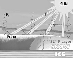
Figure 10.2 The energy balance over a snow cover in which the solar radiation, the major melting variable, is represented by F, while the solar radiation absorbed at the top of the ice sheet is represented by F(1-a), where “a” is the albedo or reflectivity of the surface. Infrared radiational cooling (F1) is represented by the squiggly dashed lines. The meltwater either flows as a stream on top of the ice or sinks vertically through the 32-degree layer. (Drawn by Dan Lietha of AiG.)
As with the previous equations, I used minimum and maximum values for the terms in the equation. One of the most important variables in the snowmelt equation is the reflectivity of the snow, which varies from about 80 percent of the sunlight for fresh, cold snow to 40 percent or lower for wet snow. A reflectivity of 40 percent is reached after several weeks of melting. If ice is exposed at the surface, the reflectivity is further reduced to between 20 and 40 percent. In the low-altitude glaciers of Norway, the reflectivity in the melt zone has been observed to fall as low as 28 percent. So, a reflectivity for the periphery of the ice sheet of 40 percent was assumed to be a maximum value during summer melting.
Reflectivity can be lowered even more if dust from dry storms is added to the ice surface. The end of the Ice Age would bring huge dust storms, especially just south of the ice sheets. These storms would develop from the large temperature differences between polar latitudes and the subtropics. So, the ice sheet surface along the periphery most likely accumulated a large quantity of dust. After the melt season, the dust would concentrate on the snow or ice surface. Figure 10.3a–c shows three snapshots of a pile of snow after a snowstorm. As the snow melted, the debris within the snow became more and more concentrated on the surface. As a result of more concentrated debris, more sunlight was absorbed by the snow and less reflected. The reflectivity of a permanent snow cover in Japan was observed to drop as low as 15 percent in late summer due to dust from air pollution. So a 15 percent reflectivity, representing a dusty snow or ice surface, was used as the minimum reflectivity.
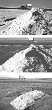
Figure 10.3a–c.
Plugging the minimum and maximum estimates for reflectivity and the other variables into the snowmelt equation, I obtained minimum and maximum estimates of melting. I averaged the two extreme melt rates for a best estimate and ended up with a melting rate of about 30 feet per year (10 m/yr).
According to this estimate, if central Michigan had an average ice depth of 2,300 feet (700 m), the ice would melt in only 75 years! Farther north, the amount of sunlight is, of course, less and the snow surface was probably less dusty. So, the ice would melt more slowly in the interior ice sheets. If the ice were of average thickness in the interior, it would take in the neighborhood of 200 years for this ice to disappear. It is expected that the melting rates for other ice sheets and mountain ice caps would correspond to those of the Laurentide ice sheet, so the total time for deglaciation would be in the neighborhood of 200 years. This is surprisingly fast — the melting would be catastrophic!
This melt time requires much less time than the uniformitarian estimates. The Flood model rate of 30 feet/year (10 m/yr) at the periphery compares very closely to modern measurements in the cool, commonly cloudy melting zones of glaciers in Alaska, Iceland, and Norway. Sugden and John2 state that glacial melting can be rapid as indicated by:
. . . many mountaineers whose tents in the ablation [melting] areas of glaciers may rest precariously on pedestals of ice after only a few days.
The present-day glaciers do not disappear at this melt rate because they are nourished by a huge amount of mountain snow in the winter that continually flows into the melting zone.
The question immediately comes up as to why uniformitarian scientists believe that ice sheets took many thousands of years to melt. The reason, like many aspects of Ice Age research, is because of their dating methods and theories, especially the astronomical theory of the Ice Age, which vastly stretches out every physical process. Mainstream scientists rarely use equations for snow and ice melt; they depend instead on their assumption of a long time-period.
All indications are that a melting rate of 30 feet/year (10 m/yr) of ice is reasonable along the periphery. Such a melting rate in a cool Ice Age climate has ominous consequences for theories and models that depend upon the uniformitarian assumption or present processes. At such a melting rate, ice sheets could not even get started within a uniformitarian climate even if a mechanism for cold enough temperatures could be found. An Ice Age simulation by Rind, Peteet, and Kukla3 started by placing 30 feet (about 10 m) of ice everywhere the ice sheet covered. Then they ran their Ice Age climate model fully expecting the ice to grow with the higher reflectivity that the snow and ice would provide in the model. Instead of growing, the 30 feet of ice melted everywhere in 5 years! The main reason is because summer sunshine is very powerful at mid and high latitudes. This experiment makes one wonder how an ice sheet could develop within the uniformitarian climate. We touched on this difficulty in chapter 3.
Putting it all together, I conclude that it took about 500 years for the Ice Age to reach its maximum and 200 years to melt. This is a total of 700 years from start to finish — a time much different than uniformitarian theories. Given the unique conditions that existed after a worldwide Flood, I have also concluded that there was only one Ice Age. It was indeed a rapid, even a catastrophic, Ice Age. It could easily have occurred between the time of the Genesis flood and the time historical records first were written in northern Europe.
Catastrophic Flooding
Is there evidence for catastrophic melting at the end of the Ice Age? Scientists have found an increasing amount of evidence of catastrophic flooding during deglaciation. One example is the Lake Missoula flood, which was rejected for over 40 years because it seemed too “biblical” (see Catastrophic deglaciation flooding by glacial Lake Missoula later in this chapter). It was finally accepted in the 1960s since the evidence for it is overwhelming.4
With the acceptance of the Lake Missoula flood, geologists have found strong evidence for catastrophic Ice Age floods in other areas of the Northern Hemisphere.5 A flood on par with the Lake Missoula flood was discovered coming out of the Altay Mountains of south-central Siberia.6 A glacier during the Ice Age had enclosed a large lake just over 1,600 feet (485 m) deep. The ice dam failed and water about 1,500 feet (450 m) deep flowed down the Chuja River Valley and eventually into the Ob River of western Siberia. Another Ice Age flood was the Bonneville flood that occurred when ancient Lake Bonneville, the largest Ice Age lake in the southwest United States, dropped about 300 feet (about 100 m) in several weeks, initiating catastrophic flooding down the Snake River of Idaho.
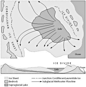
Figure 10.4. Postulated location of a lake in the vicinity of Hudson Bay and subglacial flow paths from this lake. The bottom diagram is a northeast-southwest cross section. (Redrawn from Shaw7, by Mark Wolfe.)
One of the more interesting, but speculative, Ice Age flood or floods are the subglacial (under the ice) catastrophic bursts postulated by John Shaw and other collaborators.8 Shaw, in his most radical suggestion, postulates a large lake in the vicinity of Hudson Bay that discharged about 50 times more water than glacial Lake Missoula (figure 10.4). One major pathway for the subglacial flood started in the northwest territories of Canada and passed southwest through northern Saskatchewan, ran almost the length of Alberta, and ended in northern Montana.9 A second major pathway is believed to have started around southern Hudson Bay or Labrador and flowed south into southern Ontario, the eastern Great Lakes, and New York. This later subglacial flood is believed to have carved the Finger Lakes of New York.
Of course, Shaw’s hypothesis has generated considerable controversy, especially the suggestion of a huge lake in the vicinity of Hudson Bay. After reviewing most of the evidence, I have concluded that his case is strong. If he is correct or partially correct, the current uniformitarian Ice Age paradigm needs to be almost totally rewritten to allow for a gigantic lake near Hudson Bay. He suggests that the lake had to exist near the peak of the Ice Age because flooding generally occurred when the ice boundary was close to its maximum extension. Such a large lake and catastrophic flooding when there was supposed to be a huge ice sheet over Canada is uniformitarian Ice Age heresy — at least currently. Mounting evidence is convincing many mainstream scientists that the Ice Age was very different from uniformitarian expectations.
Catastrophic Deglaciation Flooding By Glacial Lake Missoula
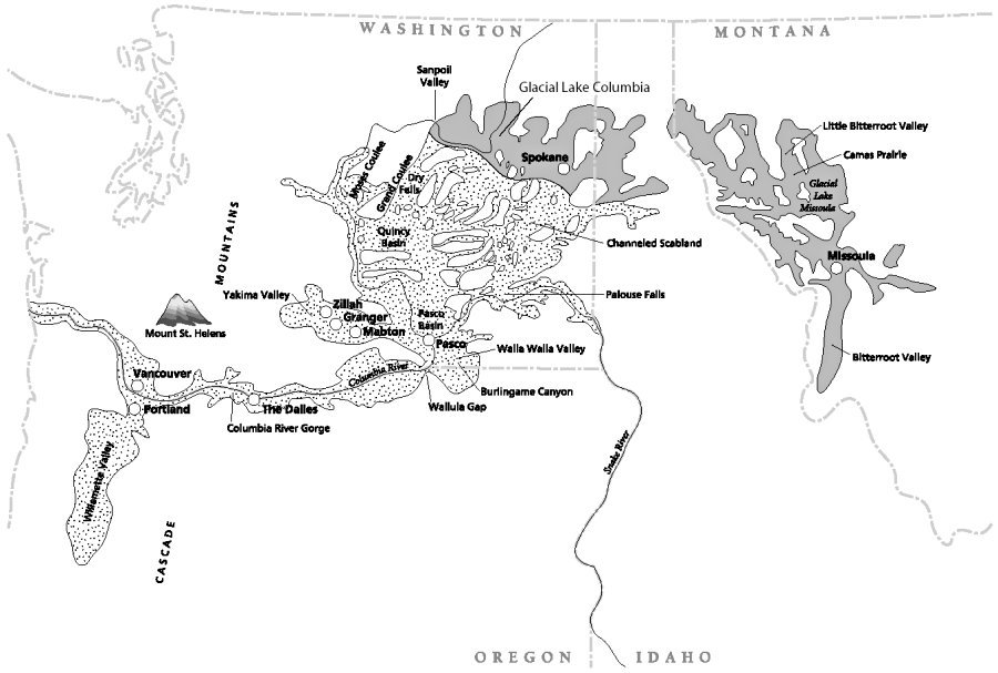
Figure 10.5. Map of the Pacific Northwest, showing the path of the Lake Missoula flood (dotted pattern) and glacial Lakes Columbia and Missoula (dark pattern). The Channeled Scabland is the part of the flood path in eastern Washington. (Drawn by Mark Wolfe.) View full-size.
Geologist J. Harlen Bretz, while examining the geology of eastern Washington in the 1920s, discovered a most unusual phenomenon. He discovered huge, deep canyons etched into hard lava. This caused him to surmise that only a flood of heretofore unheard of proportions could have formed them. The Grand Coulee had been gouged 900 feet (275 m) deep and 50 miles (80 km) long. The flood carved out the canyon where Palouse Falls is located in southeast Washington when water overtopped a lava ridge forming a canyon six miles (10 km) long and 500 feet (150 m) deep.
At first, Bretz did not understand where all this water could have originated. At the same time, J.T. Pardee postulated that a large lake existed in western Montana that was dammed by a lobe of the Cordilleran ice sheet in northern Idaho. Bretz finally made the connection and dubbed it the Lake Missoula or Spokane flood. Figure 10.5 shows glacial Lake Missoula in western Montana and the path of the Lake Missoula flood through the Pacific Northwest.
Geologists of that era were not prepared to hear of such a catastrophe. It seemed too much like the biblical flood against which they had a strong bias, so Bretz’s idea was severely challenged. For 40 years the geological establishment criticized his idea and made up other theories that, today, seem farfetched. Finally, in the 1960s, with the advent of aerial photography and better geological work, Bretz’s “outrageous hypothesis” was verified.
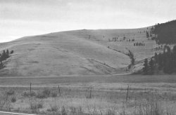
Figure 10.6. Shorelines of glacial Lake Missoula along the edge of the Little Bitterroot Valley, 75 miles (120 km) northwest of Missoula, Montana.
At the peak of the Ice Age, thick ice filled the Lake Pend Oreille River Valley in northern Idaho blocking the Clark Fork River. Meltwater from the ice flooded the valleys of western Montana, gradually filling them until they could hold no more. It had risen to about 4,200 feet (1,280 m) above sea level, based on abundant shorelines observed in the valleys of western Montana, most notably the hills east and northeast of Missoula (figure 10.6). The water depth was 2,000 feet (600 m) at the ice dam. The lake contained 540 cubic miles (2,200 cubic km) of water, half the volume of present day Lake Michigan.
Glacial Lake Missoula burst through its ice dam, probably in a matter of hours, and roared over 60 mph (30 m/sec) in places through eastern Washington into the Columbia Gorge and emptied into the Pacific Ocean. It was 450 feet (135 m) deep when it rushed over Spokane, Washington. It eroded 50 cubic miles (200 cubic km) of hard lava and silt from eastern Washington. Scoured-out lava over eastern Washington resembles a large braided stream from satellite pictures, although the stream had to have been 100 miles (160 km) wide!
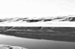
Figure 10.7. A gravel bar along the Snake River, Washington, from the Lake Missoula flood.
Much of the basalt rock has been rolled into huge gravel bars that are commonplace over the very dry scablands of eastern Washington. They look like normal gravel bars found in rivers, but on a stupendous scale. One near the Columbia River south of Vantage, Washington, is 20 miles (32 km) long and about 100 feet (30 m) high. Another bar is 300 feet (90 m) high and fills up portions of the Snake River Valley (figure 10.7). The rushing water scoured the lava so badly that it formed the lava badlands near Moses Lake, Washington.
As the Flood water came to the narrow constriction through the Horse Heaven Hills, called Wallula Gap, it backed up and formed a lake 800 feet (245 m) deep. From there, the waters rushed up the surrounding valleys, including the Walla Walla and Yakima River Valleys. The rushing water formed a series of repeating beds of sand and silt called rhythmites. Bretz noticed these unusual deposits lying on top of lava flows and included them in his evidence for the Lake Missoula flood. The best outcrop is found in Burlingame Canyon in the Walla Walla Valley (figure 10.8). The canyon was cut in about one week by water diverted from an irrigation canal, exposing the series of rhythmites. Thirty-nine of these sand and silt couplets have been counted and have inspired several theories on how they formed during the Lake Missoula flood.
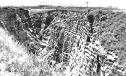
Figure 10.8. Burlingame Canyon, south of Lowden, Walla Walla Valley, Washington. Note the layered rhythmites on the sides of the canyon.
As the muddy water churned down the Columbia River Gorge, the flood enlarged the gorge between The Dalles and Portland, Oregon. Leaving the gorge, it spread out in the wide lowlands of the Willamette Valley, depositing a layer of silt rhythmites about 50 feet (15 m) thick and laying a huge gravel bar in the Portland area that is 400 feet (120 m) deep and covers 200 square miles (500 square km). The water continued racing toward the Pacific Ocean where it carved a small canyon in the continental slope. It took about a week for Lake Missoula to empty.
Strewn all along the flood path are large erratic boulders that could have only been floated in by icebergs. Most of the boulders are granite from outcrops in northern Idaho and northern Washington. One found in the central Willamette Valley attests to the power of icebergs to transport boulders during the Lake Missoula flood. Originally it weighed 160 tons (145,000 kg), before tourists broke off pieces for souvenirs. Today the rock is only 90 tons (82,000 kg). A rock of this size and composition could not have been rolled into place by water. It is composed of argillite, a slightly metamorphosed shale that is too delicate to take the rigors of water transport. Its nearest possible source is in extreme northeastern Washington. Argillite is also abundant in northern Idaho and western Montana. The boulder had to have been transported at least 500 miles (800 km). Ice rafting during the Lake Missoula flood is the only reasonable explanation.
Geologists today overwhelmingly accept the Lake Missoula flood. Before, they had trouble believing there was a flood of these proportions; later many debated how many such floods took place during the Ice Age. In the 1980s, opinion swayed from one or a few floods to anywhere between 40 and 100. The rhythmite layers found in Burlingame Canyon have played a key role in this controversy. A recent analysis of most of the data has revealed that there probably was just one Lake Missoula flood, similar to what Bretz originally believed.10
Frozen in Time
Author Michael Oard gives plausible explanations of the seemingly unsolvable mysteries about the Ice Age and the woolly mammoths.
Read Online Buy Book
Master Books has graciously granted AiG permission to publish selected chapters of this book online. To purchase a copy please visit our online store.
Footnotes
- Oard, M.J., An Ice Age Caused by the Genesis Flood, Institute for Creation Research, El Cajon, CA, p. 114–119, 217–223, 1990. Peixoto, J.P. and A.H. Oort, Physics of climate, American Institute of Physics, New York, 1992.
- Sugden, D.E., and B.S. John, Glaciers and landscape: A geomorphological approach, Edward Arnold, London, p. 39, 1976.
- Rind, D., D. Peteet, and G. Kukla, Can Milankovitch orbital variations initiate the growth of ice sheets in a general circulation model? Journal of Geophysical Research 94(D10):12,851–12,871, 1989.
- Oard, M.J., The Missoula Flood Controversy and the Genesis Flood, Monograph No. 13, Creation Research Society, Chino Valley, AZ, 2004.
- Ibid., pp. 59–67.
- Baker, V.R., G. Benito, and A.N. Rudoy, Paleohydrology of late Pleistocene superflooding Altay Mountains, Siberia, Science 259:348–350, 1993. Carling, P.A., Morphology, sedimentology, and palaeohydraulic significance of large gravel dunes, Altai Mountains, Siberia, Sedimentology 43:647–664, 1996.
- Shaw, J., B. Rains, R. Eyton, and L. Weissling, Laurentide subglacial outburst floods: Landform evidence from digital elevation models, Canadian Journal of Earth Sciences 33:226, 1996.
- Sharpe, D.R., and J. Shaw, Erosion of bedrock by subglacial meltwater, Cantley, Quebec, Geological Society of America Bulletin 101:1011–1020, 1989. Shaw, J., and R. Gilbert, Evidence for large-scale subglacial meltwater flood events in southern Ontario and northern New York state, Geology 18:1169–1172, 1990. Shoemaker, E.M., Water sheet outburst floods from the Laurentide ice sheet, Canadian Journal of Earth Sciences 29:1250–1264, 1992. Shoemaker, E.M., Subglacial floods and the origin of low-relief ice-sheet lobes, Journal of Glaciology 38(128):105–112, 1992. Gilbert, R., and J. Shaw, Inferred subglacial meltwater origin of lakes on the southern border of the Canadian shield, Canadian Journal of Earth Sciences 31:1630–1637, 1994. Sjogren, D.B., and R.B. Rains, Glaciofluvial erosional morphology and sediments of the Coronation — Spondin Scabland, east-central Alberta, Canadian Journal of Earth Sciences 32:565–578, 1995. Shaw, J., Subglacial erosional marks, Wilton Creek, Ontario, Canadian Journal of Earth Sciences 25:1256–1267, 1988. Shaw, J., A meltwater model for Laurentide subglacial landscapes; in: Geomorphology Sans Frontière. S.B. McCann (Ed.), John Wiley & Sons, New York, pp. 181–236, 1996. Shaw, J., B. Rains, R. Eyton, and L. Weissling, Laurentide subglacial outburst floods: Landform evidence from digital elevation models, Canadian Journal of Earth Sciences 33:226, 1996. Brennand, T.A., J. Shaw, and D.R. Sharpe, Regional-scale meltwater erosion and deposition patterns, northern Quebec, Canada, Annals of Glaciology 22:85–92, 1996. Kor, P.S.G., and D.W. Cowell, Evidence for catastrophic subglacial meltwater sheetflood events on the Bruce Peninsula, Ontario, Canadian Journal of Earth Sciences 35:1180–1202, 1998. Munro-Stasiuk, M.J., Evidence for water storage and drainage at the base of the Laurentide ice sheet, south-central Alberta, Canada, Annals of Glaciology 28:175–180, 1999. Beaney, C.L., and J. Shaw, The subglacial geomorphology of southeast Alberta: Evidence for subglacial meltwater erosion, Canadian Journal of Earth Sciences 37:51–61, 2000.
- Rains, B., J. Shaw, R. Skoye, D. Sjogren, and D. Kvill, Late Wisconsin subglacial megaflood paths in Alberta, Geology 21:323–326, 1993.
- Shaw, J., et al., The channeled Scabland: Back to Bretz? Geology 27(7):605–608, 1999. Oard, M.J., Only one Lake Missoula flood, TJ 14(2):14–17, 2000. Oard, M.J., The Missoula Flood Controversy and the Genesis Flood, Monograph No. 13, Creation Research Society, Chino Valley, AZ, 2004.


Support the creation/gospel message by donating or getting involved!

Answers in Genesis is an apologetics ministry, dedicated to helping Christians defend their faith and proclaim the good news of Jesus Christ.
- Customer Service 800.778.3390
- © 2024 Answers in Genesis