A Discussion of Stellar Nucleosynthesis

Introduction

In 1835 the French philosopher Auguste Comte opined that while we can learn much about the stars, their composition would forever be unknown to us. Of course, Comte was limited in his thinking by the assumption that only traditional laboratory analysis could reveal chemical composition. Ironically, about the time that Comte wrote this, new discoveries in spectroscopy were beginning to show that chemical analysis was possible over the vast distances of space. By the end of the nineteenth century, astronomers were able to identify elements present in stars. The development of astrophysics in the early twentieth century led to detailed chemical analysis of many stars. Today we know the chemical composition of many thousands of stars. Spectroscopy also allows us to determine the composition of the surfaces of planets, their satellites, and asteroids, as well as the composition of matter thinly distributed in space (the interstellar medium and the intergalactic medium). We also know the gross composition of galaxies, which represents the average composition of the stars contained by those galaxies. These studies also yield composition gradients within galaxies.

I must emphasize that in regard to stellar composition we know only the composition of the stellar photosphere, the outermost layer of a star from which nearly all light emanates. Astronomers generally assume that a star begins in a thoroughly mixed state so that its photosphere represents the star’s original composition. Astronomers further believe that normally there is not much transport of matter from the core of a star to its photosphere. Stars derive most of their energy from nuclear reactions in their cores, which over great time will alter the composition of their cores. But since stars generally do not transport material from their cores to their photospheres, this change in core composition usually will not be reflected in photospheric composition.1

A spectroscope takes the light collected by a telescope, and passes that light through a narrow slit. Behind the slit there is a dispersing element. Spectroscopes originally used prisms for this, but nearly all spectroscopes today use diffraction gratings. Diffraction gratings have several advantages over prisms. The primary advantage is that diffraction gratings can be optimized for particularly high resolution, that is, with greater dispersion in wavelength. The dispersing element spreads the light out into a multi-wavelength image of the slit. If a source produces light at a single wavelength, then its spectrum will appear as a single wavelength image of the slit. Normally a spectrum is displayed with wavelength plotted along the horizontal axis, so this image would be a vertical line, so we call the image of the slit a spectral line. A hot gas at low pressure produces a series of emissions at discrete wavelengths as the electrons in the atoms of the gas fall from higher to lower orbits. Hence, the spectrum of a hot, low pressure gas has a series of emission lines. We call this an emission spectrum. Emission spectra are seen in hot gases in space, such as the solar chromosphere, a thin layer lying above the solar photosphere. Another example would be HII regions, gas clouds primarily made of hydrogen surrounding certain hot, bright stars.

A hot gas at high pressure produces a continuous spectrum (as do hot solids and liquids). A continuous spectrum lacks emission lines, for the light is spread as a function of wavelength with a broad peak at some wavelength. Continuous spectra are good approximations to ideal blackbodies, and they follow the Stefan-Boltzmann law and Wein’s law. This later relation allows us to measure the temperature of a body emitting a continuous spectrum, for the peak wavelength of emission is inversely proportional to the temperature. Much of the interior of a star is hot gas at high pressure, and so a star’s interior produces a continuous spectrum. Thus, to a good approximation, a star is an ideal blackbody, and we can use Wein’s law to determine its temperatures.2 However, the temperature and pressure within a star decrease with increasing radius, so we view the radiation emerging from a star’s interior through the cooler, lower pressure outer layers of the photosphere. The photosphere removes light from the continuous spectrum coming from below as the electrons in the atoms of the photosphere absorb radiation and jump to higher orbits. This is the reverse process of how an emission spectrum forms, and so there are dark absorption lines superimposed upon the continuous spectrum. We call this an absorption spectrum, and this is the type of spectrum that nearly all stars produce (there are a few rare Wolf-Rayet stars that have emission lines as well). These spectral lines are the primary reason why stellar spectra slightly depart from an ideal blackbody spectrum. The wavelengths of the absorption lines are the same as the wavelengths of lines produced in emission, and each element produces a unique set of spectral lines, so identification of the elements within stars is certain in most cases. Cool stars tend to have many absorption lines, so crowding of the lines can make element identification in cool stars difficult.

We can produce all three types of spectra, continuous, emission, and absorption, in the laboratory, and so we can directly test the conditions under which various spectral lines are produced. For instance, spectral lines are subject to the Doppler Effect, so we can measure how fast astronomical sources are approaching or receding from us, as well as rotational motion. Doppler motion also arises from the motion of gas particles moving in stellar photospheres as they absorb energy to produce dark lines; this gives rise to spectral broadening. Strong magnetic fields in the presence of the formation of spectral lines will produce splitting of certain spectral lines (the Zeeman Effect). The Zeeman Effect allows us to determine the strengths of magnetic fields and polarities present where the spectral lines are formed. Astronomers use this to map the sun’s magnetic field and observe how the field changes throughout the sunspot cycle. We have evidence of strong magnetic fields present in some stars.

Exactly which spectral lines form and how strong those lines are depend upon how much of an element is present, but more importantly, also depend upon the temperature of the star. These factors allow us accurately to measure the temperature and the composition in an emitting region. Therefore, we have much confidence in the measured abundance of stellar photospheres. We also can use these principles to probe the composition and conditions of the interstellar and intergalactic media. Here the (generally cooler) clouds of gas are viewed in front of more distant sources, such as stars, galaxies, and quasars. We see solar system objects by the sunlight that they reflect, so to a good approximation the spectra of solar system objects are solar spectra. However, superimposed upon these are spectral features from the surfaces from which they are reflected, so we can use this information to infer something about the composition of these objects. For instance, the spectra of asteroids and Pluto reveal something about their surface composition.

Molecules also produce emission and absorption spectra. However, molecular spectra are much more complicated than atomic spectra, because they are dominated by many closely spaced lines due to rotational and vibrational modes within the molecules. These closely spaced lines often blend into broad spectral features. The photospheric temperatures of most stars are too hot for molecules to exist, so molecular absorption lines are present only in the coolest stars. More than a hundred molecules have been identified in the interstellar medium, normally from their emission lines at wavelengths longer than visible. For a partial list of molecules found in space, see Mathis (2000, p. 534).

In the latter half of the twentieth century, astronomers began compiling the composition of the solar system and of the universe with regards to the abundances of the elements and sometimes even within the various isotopes of the respective elements. The solar system abundance is a composite of the sun’s composition and the composition of carbonaceous chondrite meteorites, what astronomers think are the most primitive meteorites. These allegedly primitive meteorites are parts of asteroids that have fallen on the earth and hence can be examined in the laboratory. The carbonaceous chondrites are supposed to be among the least reworked of solar system objects and hence are hypothetically good probes of the original composition of the cloud of gas from which the sun and the rest of the solar system are supposed to have formed. Of course, this is an evolutionary assumption. There is diversity of composition amongst solar system objects that is explained by differentiation via various mechanisms. For instance, while the compositions of the earth and moon have some similarities, there are differences. The moon is depleted in volatiles and siderophile (iron-loving) elements compared to the earth, but it is enhanced with refractory elements (Corliss 1985, pp. 116–117). And the earth and moon are different from other planets and satellites in the solar system. The inferred cosmic abundance is a composite of stellar composition and some interstellar composition. The cosmic and solar system abundances are similar, but, as within the solar system, there are some subtle differences that normally are attributed to the unique characteristics of the primordial cloud from which the solar system supposedly formed.

The Naturalistic Origin of the Elements

Astronomers have endeavored to explain the composition of the universe via a theory of how the elements formed. The only discussion of this theory in the creation literature thus far is that of Wilt (1983). In this paper I expand upon that discussion.

Astronomers recognize two distinct episodes of element creation: primordial nucleosynthesis and stellar nucleosynthesis. Stellar nucleosynthesis also involves nucleosynthesis in supernovae. Primordial nucleosynthesis is the production of certain elements from the big bang model. The primordial elements include hydrogen, helium, and a small amount of lithium. All other elements (including some helium) are thought to have been produced in stars (normal stellar nucleosynthesis and supernovae), though a very small amount of some isotopes can be produced by spallation reactions in the interstellar medium. For a while, astronomers thought that nearly all elements originated from primordial nucleosynthesis, but it was largely the work of the late Sir Fred Hoyle in the 1950s that showed that this was not possible. The problem is that hydrogen fuses into helium at a much lower temperature than the temperatures required to synthesize helium into heavier elements. The fusion of heavier elements requires that helium first exist. In a big bang universe, by the time that the temperature had cooled sufficiently for helium to form, the window of opportunity for fusing heavier elements had closed. Only after stars had formed were temperatures recreated that could synthesize those heavier elements.

Primordial nucleosynthesis supposedly produced six isotopes: the two isotopes of hydrogen (¹H and ²H), the two isotopes of helium (³He and ⁴He) and the two isotopes of lithium (⁶Li and ⁷Li). The exact amount of lithium produced is difficult to determine. The observed abundance of the isotopes must be compared with the model predictions, but lithium is readily consumed by nuclear reactions at relatively low temperatures found in the interiors of stars, and forming stars are mostly convective, so that stellar lithium is consumed early in stars’ lifetimes. And there are a number of mysteries surrounding lithium in stars. The observed lithium abundances of many stars do not match the abundances expected from big bang cosmology, stellar structure, and nuclear physics. In addition, the sun’s lithium abundance is far lower than most stars, which for a long time suggested that the sun was unique, but in recent years a few stars with similar lithium abundances have been found. Supporters of the big bang frequently claim that the abundances of the three lightest elements predicted by the big bang model match the observed abundances, but there are several problems with this claim. First, there is much interpretation that must go into the comparison, such as the rate at which lithium has been consumed since the big bang, as just mentioned. Second, there are some discrepancies, as just mentioned. Third, the actual abundances predicted by the model depend upon some of the inputs of the model; if those inputs are altered, the predictions are altered. Essentially, the model parameters have been constrained in such a way to produce the observed abundances of the lighter elements. That is, the model has been adjusted to match the data. This is an acceptable method of constraining a model, but it is improper to claim this as evidence for the model.

If one supposes that the lighter elements were created in the big bang, the next step is to consider stellar nucleosynthesis as the source of the heavier elements. Astronomers generally credit Atkinson and Houtermans (1929) as the first to publish a paper clearly to suggest nucleosynthesis as the source of stars’ energy. Progress on this theory continued for 25 years before a clear picture emerged. Modern concepts of stellar structure and evolution began to take shape in the 1950s, with the first textbooks on the subject appearing about that time. For instance, probably the earliest such textbook is that of Schwartzschild (1958). Of supreme importance in the development of this theory was the groundbreaking paper by Burbidge, Burbidge, Fowler, and Hoyle (1957) (usually referred to in the literature by the initials, BBFH). BBFH showed the way in the various nuclear reactions that could power stars at different times and different conditions. Given that BBFH was published more than a half century ago and that much of the required nuclear data were poorly known at that time, it is amazing that this paper still is considered essentially correct in every major way. While there have been more recent reviews of the various processes of stellar nucleosynthesis (Meyer 1994; Meyer, Brown, and Luo 1996; Wallerstein, et al 1997), the principles have remained in place.

Through a process not really understood, astronomers think that stars form from clouds of gas. Early in the universe, stars supposedly formed much more rapidly than they do today, though the reason for this isn’t understood either. Astronomers really don’t know how stars form, and there are physical reasons why star formation cannot easily happen. A good, thorough review of this subject from a creation perspective would be desirable, because much work on star formation now exists in the astronomical literature. However, for our purposes here, we will let that go and grant that stars somehow formed.

A star is a large self-gravitating sphere of gas that produces energy by thermonuclear reaction in or near its core. Following normal laws of physics, we understand that the greatest pressure and temperature exist in the core of a star. Calculation using those physical laws reveals that the temperature and pressure in a star’s core is sufficient to sustain thermonuclear reactions. Since the temperature is so high in stellar cores (many millions of Kelvin), atoms do not exist there. Instead, much of a star’s interior consists of nuclei of atoms and free electrons. Most stars derive their energy from the fusion of hydrogen into helium. This is accomplished by several different pathways, but the net result is that four hydrogen nuclei fuse into one helium nucleus (⁴He). The mass of four inputted hydrogen nuclei is 0.7% more massive than a single output ⁴He nucleus. This mass defect converts into energy using the famous E = mc² equation. Using simple assumptions and this energy source, we find that the sun can shine by this mechanism for about 10 billion years. The luminosities of stars vary greatly, with the more massive stars being brighter. Stellar luminosity is a steep function of mass (approximately the fourth power of mass), but the amount of nuclear fuel available is a linear function of mass. Therefore, high mass stars have relatively short lifetimes (on the order of a million years), while low mass stars have the longest lifetimes (on the order of a hundred billion years, much older than the 13.8 billion big bang age for the universe).

Is there any evidence that thermonuclear reactions are the source of the sun’s energy (and by extension, the source of other stars’ energy)? Yes, we have at least two reasons. First, we have a very good understanding of nuclear physics, and the likely conditions in the sun’s core make it inevitable that nuclear reactions occur in the sun’s core. Some recent creationists wish to deny that the sun’s core temperature is high enough to sustain nuclear reactions (see, for instance, Henry 2003). This belief appears to stem from an attempt to eliminate the possibility of thermonuclear reactions as the primary source of the sun’s energy. If the sun is not powered by thermonuclear reactions, then it would almost certainly be powered by gravitational contraction, and that would preclude an age of more than 30 million years. If true, this would be a good argument for recent origin. But is it true? No, for even a simple back of envelope calculation reveals that the conditions in the solar core are sufficient to sustain nuclear reactions (Faulkner and Samec 2004). Second, since the late 1960s there have been numerous experiments measuring neutrinos from the reactions in the solar core. For three decades there was the mystery of the solar neutrino problem, that the sun appeared to be producing about one-third the neutrinos expected if the sun is powered by thermonuclear reactions. However, this mystery was solved with the 2001 experiment that showed that neutrinos oscillate between their three types. Additionally, more recent neutrino telescopes are directional, clearly showing that most of the neutrinos detected are indeed coming from the sun. With this information, we are now assured that the sun is producing nearly all, if not all, of its energy from thermonuclear fusion of hydrogen into helium. At one time the deficit in solar neutrinos was used as evidence of recent origin of the sun, but this is no longer a good argument (Newton 2002).

Initial Stellar Nucleosynthesis

I ought to mention some of the pathways responsible for fusion of hydrogen into helium within stars. Most stars fall along the main sequence of the Hertzsprung-Russell (HR) diagram (fig. 1 illustrates the HR diagram and its various branches; for more information on the HR diagram, see Faulkner and DeYoung 1991). Main sequence stars are the stars that derive their energy from hydrogen fusion within their cores. Lower mass stars, including the sun, do this by means of the proton-proton (p-p) chain, so named for the successive chain of protons (hydrogen nuclei) involved. The main reaction thought to work is three fold:

H + H → ²H + e⁺ + ν
²H + H → ³He + γ
³He + ³He → ⁴He + H + H,

where e⁺ denotes a positron (an anti-electron), ν denotes a neutrino, and γ denotes a gamma ray, a high energy photon. Of course, H and He refer to the nuclei of the hydrogen atom and helium atom, respectively. The superscripts refer to the number of nucleons in the respective nuclei, with no subscript corresponding to one. The positron and neutrino are produced as a consequence of the transmutation of a neutron into a proton in the first step—the positron is required to balance the charge, and the neutrino balances the appearance of the positron. Electrons, neutrinos, and their anti-particles are members of a class of particles called leptons. As with charge conservation, total lepton number must be conserved. For accounting purposes, we count the neutrino as a lepton and the positron as an anti-lepton so that the number of leptons sums to zero. The gamma ray is absorbed and reemitted many times which gradually degrades the energy to much lower temperature as that energy makes it way outward from the core to the photosphere where it radiates into space. The first two steps must happen twice for the third step to take place. Notice that there are a total of six protons (hydrogen nuclei) that are input into the reaction, with an output of one helium nucleus and two protons, so that the net reaction is four protons fused into one helium nucleus. This reaction probably accounts for more than 90% of the sun’s energy, with the remaining energy coming from related side reactions with the same net result.

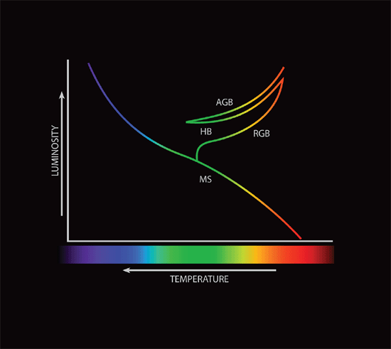
Fig. 1. The Hertzprung-Russell diagram showing stellar luminosity as a function of effective temperature. The main sequence, red giant branch, horizontal branch, and the asymptotic giant branch are indicated.

For the more massive stars on the main sequence the CNO cycle is the main reaction. The CNO cycle is so called, for it uses carbon, nitrogen, and oxygen as catalysts to fuse hydrogen into helium, but the net reaction is the same as for the p-p chain. The first six steps in the reaction are:

¹²C +mH → ¹³N + γ
¹³N → ¹³C + e⁺ + ν
¹³C + H → ¹⁴N + γ
¹⁴N + H → ¹⁵O + γ
¹⁵O → ¹⁵N + e⁺ + ν
¹⁵N + H → ¹²C + ⁴He

Notice that the ¹²C output in the sixth step goes back into the process as an input in the first step. The last step in this process has an alternate outcome:

¹⁵N + H → ¹⁶O + γ
¹⁶O + H → ¹⁷F + γ
¹⁷F → ¹⁷O + e⁺ + ν
¹⁷O + H → ¹⁴N + ⁴He

The ¹⁴N created in the fourth step of this second process can be inputted into the fourth step of the first process. As with the p-p chain, there are side reactions that also proceed, but the steps listed here provide most energy production. In the strictest sense, the CNO cycle is not a catalytic one, for while the total number of heavier nuclei is conserved, the relative numbers of the various isotopes are shuffled. In equilibrium, the CNO cycle produces a 3.5 ratio of ¹²C to ¹³C, and ¹⁴N becomes the most abundant nucleus. Red giant stars generally have abundances closer to these values than main sequence stars, which is taken as evidence that CNO products have been transported via convection from their interiors to their photospheres.

In the standard model of the big bang, there were no atoms heavier than helium suitable for fusion in the early universe, so the first massive stars must have used some version of the p-p chain rather than the CNO cycle. Where did the carbon, nitrogen, oxygen, and other heavier elements come from? Astronomers think that those elements were synthesized in stars. Stars on the main sequence are thought to derive their energy from fusion of hydrogen into helium in their cores. Therefore, once all the hydrogen fuel in a star’s core is exhausted, a star can no longer be on the main sequence. Astronomers think that at this point stars evolve off the main sequence to become red giants. Red giant stars derive energy from fusing hydrogen into helium in thin shells around their helium cores. Faulkner and DeYoung (1991) previously reviewed stellar evolution, and Faulkner (2008) reviewed stellar remnants. It the discussion that follows, far greater time than is allowed in a recent creation model is required, so it would appear unlikely that this could be incorporated easily within a biblical cosmology.

As a red giant star ages, it accumulates the helium “ash” from the fusion in the shell onto the core. Since the core has no source of energy, the accumulation of additional helium causes the core to contract and heat. Eventually the temperature in the star’s core may raise high enough to initiate the fusion of helium into carbon. This begins the horizontal branch (HB) stage. Helium fusion is accomplished by the triple alpha process, so called, because it involves three helium nuclei (a helium nucleus is called an alpha particle). The triple alpha process technically has an intermediate step:

α + α → ⁸Li.

⁸Li is unstable with a half-life of less than a second, decaying back into two alpha particles. However, if another alpha particle interacts with the ⁸Li prior to decay, then the following reaction results:

α + ⁸Li → ¹²C.

This second step must happen before the ⁸Li can decay, so the reaction does involve a nearly simultaneous reaction of three alpha particles. The net reaction is that three helium nuclei fuse into a single C nucleus. As with the fusion of hydrogen into helium, the product of this reaction has less mass than the inputs, so energy is produced by the conversion of mass into energy. However, the amount of energy released in this reaction is about 10% of the earlier reaction.

Related to the triple alpha process is alpha capture. An alpha particle may fuse with ¹²C to produce ¹⁶O:

¹²C + ⁴He → ¹⁶O + γ.

The process may repeat:

¹⁶O + ⁴He → ²⁰Ne + γ
²⁰Ne + ⁴He → ²⁴Mg + γ

and so on. Notice that these nuclei are integral multiples of an alpha particle. That is, these nuclei have atomic numbers equal to 2n and atomic masses equal to 4n, where n is a positive integer greater than 3. These are the most common isotopes of some of the most common elements. Elements produced in this manner are called alpha process elements, because astronomers explain their existence by addition of alpha particles to existing nuclei. Astronomers think that most of the alpha process elements heavier than carbon are produced in massive stars that are precursors of type II supernovae. The subsequent eruption of type II supernovae is thought responsible for spreading the alpha process elements throughout the universe. This material enriches gas clouds, from which more stars form, and the process repeats. In this way, chemical enrichment hypothetically leads to ever-increasing amounts of heavier elements in later generations of stars. The alpha process elements produced this way terminate with titanium (atomic number 22). However, astronomers think that type Ia supernovae eruptions can extend alpha capture up to iron and related elements. A type Ia supernova results from interaction of the components of a certain kind of binary star where one member is a white dwarf. Of course, type Ia supernovae eruptions supposedly can spread these more heavy nuclei into space. The alpha process generally must truncate with iron, because alpha capture up to iron is exothermic, but further alpha capture is endothermic, and there does not seem to be a suitable astrophysical environment for the efficient endothermic production of nuclei via alpha capture. The exothermic/endothermic divide is the result of iron being the most entropic nucleus with respect to binding energy.

If protons (H nuclei) are available, the fusion of protons with some of the products of successive alpha capture can produce other isotopes. The neon-sodium cycle is:

²⁰Ne + H → ²¹Na + γ
²¹Na → ²¹Ne + e⁺ + ν
²¹Ne + H → ²²Na + γ
²²Na + H → ²³Mg + γ
²³Mg → ²³Na + e⁺ + ν
²³Na + H → ²⁰Ne + He

Some have suggested that this sort of reaction, while not important in energy generation, can produce nuclei that may be significant for other reasons. For instance, the ²¹Ne produced in the second step of this reaction could be a source of neutrons in the s process.

In massive stars C and O may further fuse with themselves. For instance, there are five possible outcomes of C fusion:

¹²C + ¹²C → ²⁴Mg + γ
¹²C + ¹²C → ²³Na + H
¹²C + ¹²C → ²³Mg + n
¹²C + ¹²C → ²⁰Ne + ⁴He
¹²C + ¹²C → ¹⁶O + 2⁴He,

where n stands for a neutron. Six possible outcomes for O fusion are

¹⁶O + ¹⁶O → ³²S + γ
¹⁶O + ¹⁶O → ³¹P + H
¹⁶O + ¹⁶O → ³¹S + n
¹⁶O + ¹⁶O → ²⁸Si + ⁴He
¹⁶O + ¹⁶O → ²⁴Mg + 2⁴He
¹⁶O + ¹⁶O → ³⁰Si + 2H

In addition to direct fusion and alpha capture, other reactions are possible in massive stars. Nuclei can capture electrons via the weak force. Neutron capture also occurs, a topic that I shall discuss shortly. Furthermore, in the intense heat, density, and pressure of the core, photons from the high-energy tail of the distribution of the photons can photodisintegrate heavy nuclei. A sort of steady state is established that BBFH called the e process (e standing for equilibrium). The steady state composition of the various isotopes can be determined by a series of coupled differential equations.

Hydrogen fusion in stars normally is stable, but helium fusion is not. The fusion of helium into carbon occurs at a much higher temperature than hydrogen fusion (10⁸ K as opposed to 10⁷ K). However, a more important factor is the inability of the helium to expand as it is heated by fusion of hydrogen into helium. The helium in the core of a red giant star is primarily supported by electron degeneracy pressure rather than normal gas pressure. When energy is released in a gas supported by normal gas pressure, the gas responds by expanding and consequently cooling. Fusion reactions are extremely temperature sensitive, so this expansion has a self-regulating effect—the onset of fusion releases much heat, which slightly expands the gas, which slows the reaction rate. However, in an electron degenerate gas, increased heat does not expand the gas, so as fusion commences, the temperature quickly rises, which rapidly increases the rate of fusion. This sort of thermonuclear runaway is called the helium flash. When this happens in the core, the gas eventually gets so hot that normal gas pressure again becomes the dominant pressure, the gas cools, and the energy production rate slows. Theoretically (and in computer models), the helium flash occurs at the tip of the red giant branch on the HR diagram, and the eventual decreased energy production leads downward to the horizontal branch.

The horizontal branch represents a position of stability for some time. However, as with hydrogen fusion in the core, the helium fuel in the core eventually is exhausted. Once all the helium in the core is exhausted, the star cannot remain on the horizontal branch. The core once again contracts, causing the star’s outer layers to expand and cool, and the star ascends the asymptotic giant branch (AGB). Astronomers think that AGB stars obtain energy from the fusion of hydrogen into helium and helium into carbon in two thin concentric shells around the core. Asymptotic giant stars have been invoked to explain carbon stars and S stars, and they are thought to be significant locations of nucleosynthesis of some of the relatively rarer elements. This is thought to happen late in the AGB through episodic fusion known as thermal pulses. As the initiation of helium fusion in the core leads to the helium flash, fusion in a thin shell results in a helium flash. However, the mechanism is a bit different, because the helium shell is not electron degenerate; it merely is too thin for sufficient expansion. Since the shell cannot expand upon initiation of helium fusion, the shell rapidly heats, consumes most of the helium, and then finally expands. Astronomers think that between 10⁴ and 10⁵ years occur between thermal pulses. Thermal pulses in AGB stars yield two important things: a large number of neutrons that lead to s process nucleosynthesis, and thermal instabilities in the envelope that transport the s process products to the surface.

The s Process

What is the s process? Nuclei readily absorb any free neutrons. Since free neutrons have a relatively short half-life (a little more than ten minutes), free neutrons rapidly decay. However, if there is a source of neutrons and abundant nuclei, then the nuclei quickly capture virtually all of the neutrons. The addition of neutrons increases the atomic mass of a nucleus, but does not increase the atomic number. Thus, this process can produce heavier isotopes of an element. However, if a nucleus gains too many neutrons it becomes unstable, leading to nuclear decay. The most common form of decay is beta decay, but a few isotopes experience alpha decay. As previously mentioned, an alpha particle is a helium nucleus, so the emission of an alpha particle reduces a nucleus’ atomic number by two and its atomic mass by four. Thus an alpha decay reduces a nucleus’ identity by two in the periodic table of elements. A beta particle can be either a free electron or positron, but the s process normally results in ejection of electrons. The reason is that the s process occurs in nuclei in which the ratio of the number of neutrons to protons is too high for stability. Since the electron has negative charge, we call this negative beta decay (the ejection of a positron is positive beta decay). A neutrino also is ejected to preserve lepton number. Negative beta decay amounts to the transmutation of a neutron into a proton. This decay does not change the atomic mass of the nucleus, but it increases the atomic number, and hence increments the type of atom that the nucleus represents by one on the periodic table. If nuclei are bombarded by free neutrons at a rate that is much slower than the rate at which any unstable nuclei decay, then the unstable nuclei will decay before they can acquire additional neutrons. This is the s process (the s means slow, as it refers to the slow rate of neutron capture as compared to the decay rate).

This is in contrast to the r process (where r stands for rapid), where the nuclei are bombarded so quickly that they are far more likely to undergo additional neutron capture(s) before experiencing beta decay. The distinction is important, for the r process and s process follow different pathways to produce different isotopes.

There are a number of sources of neutrons during thermal pulses in AGB stars. One reaction responsible for neutrons is the fusion of carbon into oxygen via alpha capture:

¹³C + ⁴He → ¹⁶O + n.

A similar reaction occurs for oxygen fusion into neon:

¹⁷O + ⁴He → ²⁰Ne + n.

Earlier operation of the CNO cycle produces ¹³C and ¹⁷O for this alpha capture to work.

Another important reaction is

²²Ne + ⁴He → ²⁵Mg + n.

The CNO cycle produces a large amount of ¹⁴N, and two alpha captures can synthesize it into ²²Ne, permitting this reaction to occur. The neutron flux in a thermal pulse is sufficient to bombard many nuclei present, but not so high as to prohibit decay of any unstable nuclei produced prior to another neutron capture (otherwise, this would be r process).

We have seen that alpha capture can account for the most-common (even-numbered) elements up to iron. Though some of the isotopes lighter than iron are explained by the s process, astronomers think that there are more efficient ways to produce most of these lighter elements. However, the real strength of the s process is in explaining many of the isotopes of the transferric elements. Consider iron, which has four stable isotopes, ⁵⁴Fe, ⁵⁶Fe, ⁵⁷Fe, and ⁵⁸Fe, with ⁵⁶Fe being the most abundant isotope. Starting with ⁵⁶Fe, one or two neutron captures can produce the two heavier stable isotopes. If a third neutron is captured, a ⁵⁹Fe nucleus is produced. ⁵⁹Fe is unstable, and it beta decays into ⁵⁹Co, the only stable isotope of cobalt. The ⁵⁹Co in turn can absorb a neutron to become ⁶⁰Co, which beta decays into ⁶⁰Ni. The ⁶⁰Ni nucleus can then capture neutrons to produce some of the heavier stable isotopes of nickel. If a nickel nucleus absorbs enough neutrons that it becomes unstable, then it beta decays into another element, and the process continues. This process can account for many of the isotopes heavier than iron. The s process terminates with bismuth-209, because ²⁰⁹Bi is the heaviest stable nucleus (Clayton and Rassbach 1967). Additional neutron capture of ²⁰⁹Bi enters a loop that leads back to ²⁰⁹Bi via an alpha decay.

We can compute the equilibrium abundances of various nuclei with a series of coupled differential equations of the form

dN_A/dτ = -σ_AN_A + σ_A-1N_A-1,

where N is the number density of a particular isotope, A is the atomic mass, σ is the cross section of interaction between a neutron and a particular isotope, and τ is the neutron exposure, given by,

τ = v_T ∫ n_n(t) dt,

where v_T is the thermal velocity, and n_n is the neutron density (Clayton 1968, pp. 558–560). The set of differential equations is subject to the boundary conditions of beginning with iron-56 and terminating with bismuth-209. Simultaneous solutions of these equations lead to predictions of relative abundances of isotopes.

Of particular interest is technetium, the lightest element for which there are no stable isotopes. ⁹⁸Mo is the heaviest of the six stable isotopes of molybdenum. The s process accounts for the production of technetium-99, the longest-lived isotope of technetium. A neutron capture produces ⁹⁹Mo which then beta decays into ⁹⁹Tc. Technetium was discovered in the spectra of certain red giant stars in 1952. Astronomers think that red giants are very old, certainly far too old for the technetium they contain to be primordial. Technetium is not found in isolation; rather in the red giants where technetium is found, many other s process elements are present. The composition of these stars is so remarkable that we call them metal stars, and they are given the spectral classification S. The S spectral class is parallel in temperature to K and M spectral classes. The understanding is that the technetium and the other s process isotopes were recently produced near the cores of these stars, but then the products of this nucleosynthesis were rapidly brought to the surfaces. Stars generally do not have fully convective envelopes, but the thermal pulses inject so much energy into the envelopes of these stars that thermal pulses are accompanied by episodes of full convection. These episodes are called dredge-up. This is one of the rare exceptions where products of nucleosynthesis deep inside of stars are brought to the surface. The period between the episodes of dredge-up must be short enough that not much of the technetium can decay.

The r Process

The s process can explain many, but not all, transferric elements and their isotopes up to bismuth, as well as some of the isotopes of the elements lighter than iron. Most of the remaining elements are explained by the r process. The r process isotopes are produced when nuclei undergo neutron capture that is so rapid that unstable nuclei have insufficient time to beta decay before undergoing additional neutron capture. Obviously, the r process requires copious amounts of neutrons, far more than thermal pulses in AGB stars can produce. The neutron densities required for the s process is within a few orders of magnitude of 10⁵/cm³, while the neutron density required for the r process is within a few orders of magnitude of 10²³/cm³ (Clayton 1968, p. 557). Obviously, the conditions for these two processes are far removed from one another. The only known source of neutron densities high enough for the r process to operate is in supernova explosions. In supernova explosions the matter density is very high, and the high photon density with extremely high temperature results in much photodisintegration of nuclei and production of many free neutrons.

In the discussion of the r and s processes, it is common to plot the various nuclei of isotopes with atomic number, Z, increasing upward and the number of neutrons, N, increasing to the right. See Fig. 2 for a schematic diagram of this. Each box represents a stable nucleus, with various species of the same element appearing adjacent horizontally. The locations of unstable nuclei are not indicated, but they can be inferred by the locations of where boxes otherwise would be. For instance, the leftmost red box in Fig. 2 has six adjacent stable nuclei, but there are two adjacent unstable nuclei, one directly above, and one to the upper left. On the other hand, the topmost red box has only two adjacent stable nuclei and six adjacent unstable nuclei. Fig. 2 represents only a very small portion of the entire plot, for there are hundreds of stable nuclei. On a complete plot of all isotopes, stable nuclei form a roughly diagonal band from lower left to upper right, with radioactive isotopes surrounding the stable nuclei. As nuclei capture neutrons, they do not change their elemental identity, so they migrate horizontally to the right on the chart. In Fig. 2 neutron capture is indicated by the solid horizontal arrows. The normal decay mode of unstable nuclei is negative beta decay, in which the value of N decrements by one while the value of Z increases by one. Therefore, negative beta decay results in a nucleus moving diagonally upward to the left on the chart. Beta decays are indicated by wavy diagonal arrows. The shorter wavy arrows indicate single beta decays, while the longer ones indicate multiple beta decays.

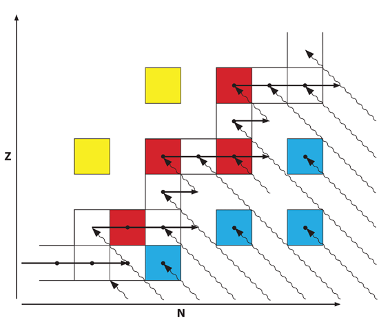
Fig. 2. Schematic diagram illustrating the r and s processes, with atomic number plotted vertically and atomic number plotted horizontally. Each block represents nuclei of a stable isotope. The horizontal solid arrows represent neutron capture, while the wavy diagonal arrows represent beta decay. The isotopes represented by white boxes result from either the s or r process. The blue boxes represent isotopes that result only from the r process, while the red boxes are s-only isotopes. The yellow boxes represent isotopes produced by proton capture.

The s process never deviates far from the diagonal band of stable nuclei. As a nucleus accumulates neutrons, it may pass through several stable nuclei, but it eventually reaches an unstable nucleus that normally beta decays before it can accumulate any more neutrons. If a stable isotope of a particular element exists two or more slots to the right of the last stable isotope, then the s process usually cannot produce that stable “stranded” isotope. As slow neutron capture repeats, the s process can proceed to ever-heavier nuclei moving along the contiguous stable isotopes of many elements. On the other hand, the r process can yield nuclei of an element that are several slots to the right of the last stable nucleus. These nuclei beta decay several times, taking them back upward to the left and toward the diagonal band of stable nuclei. Some of the stable nuclei that result from the r process also can be produced by the s process. In Fig. 2 the nuclei that can be formed by both the r and s processes are indicated by white boxes. However, r process, because it “pushes” nuclei so far to the right of the diagonal band of stable nuclei, can produce previously mentioned stranded isotopes that the s process cannot produce. In Fig. 2 these are represented by blue boxes. Since these stranded isotopes are stable, they cannot beta decay, so any stable nuclei one or more positions diagonally upward to the left cannot be produced by the r process. These isotopes are shielded from the r process, and can be produced only by the s process. In Fig. 2 these “s only” isotopes are represented by red boxes. Finally, there are some stable isotopes to the upper left of the band of stable isotopes. Since beta decay cannot lead to these isotopes, they must have originated by some other mechanism. That mechanism is by proton capture. Those nuclei are indicated with yellow boxes in Fig. 2.

Fig. 3 illustrates some real-world examples of the various processes that I’ve described. Consider ¹²⁷I, the only stable isotope of iodine, as it undergoes the s process. Starting in the white box in the lower left of Fig. 3, ¹²⁷I absorbs a neutron, becoming ¹²⁸I, which beta decays with a half-life of 25 minutes. This is well within the time constraint of the s process, so it beta decays into ¹²⁸Xe. The next four isotopes of xenon are stable, so the slow capture of neutrons can synthesize Xe isotopes up to and including ¹³²Xe (the other two stable isotopes of xenon, ¹³⁴Xe and ¹³⁶Xe, are two of the “stranded” isotopes, which I will discuss in a moment). An additional neutron capture produces ¹³³Xe, which beta decays into ¹³³Cs with a half-life of 4.27 days. ¹³³Cs is the only stable isotope of cesium. The addition of a neutron transmutes ¹³³Cs into ¹³⁴Cs, which beta decays into ¹³⁴Ba with a half-life of 2.19 years, well within the time constraint of the s process. ¹³⁴Ba is stable, as are the next four isotopes of barium, so slow neutron capture can produce the isotopes of barium through ¹³⁸Ba. The slow capture of an additional neutron yields ¹³⁹Ba, which beta decays into ¹³⁹La, with a half-life of 83 minutes. ¹³⁹La is the heavier of the two stable isotopes of lanthanum. The slow neutron capture of an additional neutron transmutes ¹³⁹La into ¹⁴⁰La, which decays into ¹⁴⁰Ce. ¹⁴⁰Ce is one of four stable isotopes of cerium, but ¹⁴¹Ce is unstable, so a slow neutron capture into ¹⁴¹Ce leads to beta decay into ¹⁴¹Pr, the only stable isotope of praseodymium. The s process continues on beyond this point, but I will end my discussion of it here.

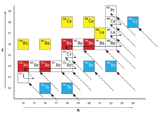
Fig. 3. Illustration of the r and s processes operating in the vicinity of xenon, cesium, barium, lanthanum, cerium, and praseodymium.

In Fig. 3, the described path of the s process from iodine to praseodymium is indicated by the arrows passing through the white and red boxes. To the upper left of this track there are two isotopes of barium (¹³⁰Ba and ¹³²Ba), one isotope of lanthanum (¹³⁸La), and two isotopes of cerium (¹³⁶Ce and ¹³⁸Ce). These isotopes obviously could not form via the s process. Instead, they formed through proton capture. The boxes representing these isotopes are yellow. To the lower right of the track followed by the s process there are five “stranded” isotopes indicated in blue, two isotopes of tellurium (¹²⁸Te and ¹³⁰Te), two isotopes of xenon (¹³⁴Xe and ¹³⁶Xe), and one isotope of cerium (¹⁴²Ce). They obviously cannot form via the s process, so they must have formed from the r process. The rapid accumulation of protons on a nucleus usually results in negative beta decay, or in multiple negative beta decays. As with beta decay in the s process, each beta decay in the r process moves a nucleus diagonally upward and leftward. The tracks that various nuclei can follow as they beta decay from the r process are shown as wavy diagonal lines in Fig. 3. Since many of the parent isotopes that beta decay in the r process can be quite over-heavy in neutrons, many of them lie off the bottom or to the right of the figure.

Notice that not only can the r process explain the five isotopes to the lower right of the red path that the s process cannot explain, but the r process also can produce many of the same isotopes that the s process can. The boxes representing these isotopes are white. However, there are a few isotopes along the path of the s process that the r process cannot produce. In Fig. 3 those isotopes are ¹²⁸Xe, ¹³⁰Xe, ¹³⁴Ba, and ¹³⁶Ba, and they are represented by red boxes. The r process cannot produce these isotopes, because these isotopes are shielded by other, stable isotopes. For instance, ¹²⁸Te lies two spaces diagonally to the lower right from ¹²⁸Xe. Since ¹²⁸Te is stable, it is not possible for a beta decay to lead through it to get to ¹²⁸Xe. ¹³⁰Te similarly shields ¹³⁰Xe, as ¹³⁴Xe shields ¹³⁴Ba, and ¹³⁶Xe shields ¹³⁶Ba. Hence, these four isotopes, in red, are considered s-only isotopes. The five isotopes in blue are considered to be r-only isotopes. As previously mentioned, the five p only isotopes are yellow. As you can see, most isotopes can result from either the s process or the r process.

Discussion

Armed with these considerations, knowledge of nuclear cross sections, and some understanding the physical conditions present in the environments under consideration, it is possible to establish a set of coupled differential equations of the type previously discussed. There is one differential equation for each isotope, so there are many of these coupled differential equations, which require a sophisticated computer program to solve. One must impose boundary conditions. For the s process, one normally assumes that the s process becomes significant with the iron group of elements and terminates with lead. Astronomers think that they have a good understanding of the environments in which the s process operates. The r process is a bit more complicated for several reasons. One reason is that the astrophysical environments where the r process is significant are a less well-known than those in which the s process operates. This is indicated by the far greater number of papers in recent years addressing the r process than the s process. Just a few examples of recent r process papers are Boyd et al (2012), Meyer and Brown (1997), and Ning, Qian, and Meyer (2007). Another complication of the r process is that it does not terminate at lead and hence includes more isotopes, but the yield decreases dramatically at higher atomic number and goes to zero as the trans-uranic elements are reached. More importantly, for isotopes that can be produced by both the r and s processes, the effects of the s process must be subtracted to find the amount of nuclei of each isotope resulting from the r process alone. Additionally, there are a number of simplifying assumptions made along the way that introduce a small amount of error.

Ultimately, it is possible to compute predictions of the amounts of each isotope that one would expect from this theory of stellar nucleosynthesis. There is difficulty in comparing the predictions with actual data. Tabulations of the composition of the universe have been done for many decades. One of the more recent tabulations is that of Däppen (2000, pp. 29–31), which in turn was compiled from several sources. Most of these tabulations don’t separate the various isotopes of the elements, but rather they list the abundance of each element with all isotopes combined. The tabulations are of several distinct sets. One set is the terrestrial abundance. Another set is the solar system abundance. This normally is determined from solar composition, particularly of the volatile elements, but also from meteorites for the more refractory elements. Then there is a cosmic abundance, which is a composite of stellar composition derived from spectroscopy. While there are similarities between these sets, there are differences. The differences are explained by fractionalization of terrestrial material and differences in origin of matter for various stars as compared to the solar system. Within the caveats of these variations due to history and some range in the computed isotopic abundances, there is qualitative agreement between the theory of stellar nucleosynthesis and observed abundances. This is taken as confirmation that the theory of the creation of isotopes through stellar nucleosynthesis is correct.

This is the ultimate evolutionary theory—the universe began in a big bang, but only a few of the lightest elements were made then. Most of the elements necessary for life were synthesized in stars that then through winds or explosions spread that material in space, and the earth and solar system and eventually our bodies formed from the elements created in stars. Many astronomers, such as Harlow Shapley, Carl Sagan, and Neil DeGrasse Tyson are quoted as saying that we are made of star stuff. More recently Lawrence Krauss has mockingly said, “Forget Jesus. The stars died so you could be here today.”3

A good theory must have good explanatory power. That is, a theory must explain what we already know. In a qualitative sense the theory of stellar nucleosynthesis does this. It can explain the composition of the current universe. However, the fact that there is variation in composition within the solar system and among stars clearly indicates that this is not an exact science. Any variation is explained in terms of local differences in history, either with different composition generated locally or with physical separation occurring locally. For instance, the earth and moon supposedly formed from the same pre-solar nebula. The earth and moon share some similarities in composition, but they also have marked differences—the moon is deficient in heavier elements as compared to the earth. This generally is explained by the origin of the moon, with the current favored theory that the moon resulted from a grazing incidence collision of the earth with a Mars-sized object. Similarly, the terrestrial planets have far less of the lighter elements than the Jovian planets do. This is explained by the early sun heating and removing the lighter elements from the inner solar system, but not the outer solar system. Similarly, while the terrestrial planets have similar composition, there are large differences, and the Jovian planets are likewise. Again, this is explained in terms of slightly different histories.

Or consider S stars. S stars are a particular class of red giant stars that have chemical abundances that are markedly different from other red giant stars. S stars contain excess zirconium and other metals that are thought to be products of the s process. This is interpreted as S stars being AGB stars with thermal pulses providing neutron flux for the s process, as well as consequent thermal pulses leading to deep convection to dredge up the products of the s process to the photospheres of S stars. Related to S stars are barium stars, so called because of their prominent spectral lines due to barium. Astronomers invoke close binary interactions to explain barium stars. Also related to S stars are carbon stars, which are red giants with an anomalous amount of carbon. Carbon stars stand out because by far they are the reddest stars. Cosmically, oxygen is more abundant than carbon, and most stars reflect this abundance. Red stars are cool enough for some molecules to exist in their atmospheres. In red giants with normal chemical abundance, all of the carbon is consumed in CO, leaving the excess oxygen to form metal oxides. However, in carbon stars all of the oxygen is consumed in the CO, which frees up both carbon and metals. The dominant factor in making carbon stars so red is the huge amount of absorption of blue and violet light by the metals. Many other types of stars are explained by similar reasoning. But once the process of explaining differences begins, virtually any differences can be explained, all the while defending the basic paradigm. These sorts of musings eventually take on the characteristics of just-so stories that we so often encounter in evolutionary explanations. A theory that explains anything and everything explains nothing.

But in addition to having explanatory power, a good theory also must have predictive power. That is, a good theory must not only explain what we know, but it ought to anticipate and hence predict some things that we don’t yet know. It does not appear that the detailed theory of primordial and stellar nucleosynthesis makes such predictions. That is, the power of nucleosynthesis theory in astronomy is entirely explanatory.

Conclusion

I have briefly reviewed the theory of stellar nucleosynthesis for the recent creation community. Of particular interest were the r process and s process. My purpose has been to educate others in some of the details of this theory, and perhaps to stimulate further discussion. While the theory appears robust in its explanatory power, one could question how well it explains known chemical abundances. A study to answer this question would be very involved, requiring tremendous computational detail. Even if more detailed studies confirmed that the theory has good explanatory power, this is far less convincing than predictive power. At this time, it does not appear that the theory of nucleosynthesis has any predictive power. Henry (2006) reached a similar conclusion about primordial nucleosynthesis.

Can we develop a creationary model to explain the chemical composition of the universe? Perhaps. Much of the Creation Week was miraculous, or at least outside of the realm that science today is equipped to probe, so one could posit that God created the elemental abundances pretty much as they exist today. However, many will find such an answer unsatisfactory, particularly if there is no clear standard of design of the elemental composition. On the other hand, God could have used physical processes as we now understand them. That is, God could have ordained physical processes to operate to produce the elemental abundances that we see in the universe. Of course, in a biblical framework, this must have happened very rapidly, far more rapidly than the gradual processes described here. There have been a few initial attempts to account for chemical abundances in the creation literature in such a physical way. In the initial concept of his white hole cosmology, Humphreys (1994) proposed rapid primordial nucleosynthesis of elements. Boudreaux (2012) and Davies (2013) have proposed similar things. However, all of these suggestions are at best preliminary. I encourage further development of ideas of this type.

References

Atkinson, R. d’E., and F. G. Houtermans. 1929. Zur frage der aufbaumöglichkeit der elemente in sternen. Zeitschrift für Physik. 54:656–665.
Boudreaux, E. A. 2012. God created the earth. Denver, Colorado: Rocky Mountain Creation Fellowship.
Boyd, R. N., M. A. Famiano, B. S. Meyer, Y. Motizuki, T. Kajino, and I. U. Roederer. 2012. The r-process in metal-poor stars and black hole formation. The Astrophysical Journal Letters 744:L14 (4pp.).
Burbidge, E. M., G. R. Burbidge, W. A. Fowler, and F. Hoyle. 1957. Synthesis of the elements in stars. Reviews of Modern Physics 29, no. 4:547–650.
Clayton, D. D. 1968. Principles of stellar evolution and nucleosynthesis. New York, New York: McGraw-Hill.
Clayton, D. D., and M. E. Rassbach. 1967. Termination of the s-process. Astrophysical Journal 148:69–85.
Corliss, W. R. 1985. The moon and the planets: A catalog of astronomical anomalies. Glen Arm, Maryland : Sourcebook Project.
Däppen, W. 2000. Atoms and molecules. In Allen’s astrophysical quantities, ed. A. N. Cox, pp. 27–51. 4th ed. New York, New York: Springer-Verlag.
Davies, K. 2013. Counting back to zero: A review of cosmological models that begin under conditions of zero entropy. In Proceedings of the Seventh International Conference on Creationism, ed. M. Horstemeyer. Pittsburgh, Pennsylvania: Creation Research Fellowship.
Faulkner, D. R. 2008. A review of stellar remnants: Physics, evolution, and interpretation. Creation Research Society Quarterly 44, no. 2:76.
Faulkner, D. R. and D. B. DeYoung. 1991. Toward a creationist astronomy. Creation Research Society Quarterly 28, no. 3:87–92.
Faulkner, D. R. and R. G. Samec. 2004. Helioseismology—a reply to Jonathan Henry. Creation Research Society Quarterly 40, no. 4:210–215.
Henry, J. F. 2003. Helioseismology: Implications for the standard solar model. Creation Research Society Quarterly 40, no. 1:34.
Henry, J. 2006. The elements of the universe point to creation: Introduction to a critique of nucleosynthesis theory. Journal of Creation 20, no. 2:53–60.
Humphreys, D. R. 1994. Starlight and time. Green Forest, Arkansas: Master Books.
Mathis, J. S. 2000. Circumstellar and interstellar material. In Allen’s astrophysical quantities, ed. A. N. Cox, pp. 523–544. New York, New York: Springer-Verlag.
Meyer, B. S. 1994. The r-, s-, and p-processes in nucleosynthesis. Annual Review of Astronomy and Astrophysics 32:153–190.
Meyer, B. S., and J. S. Brown. 1997. Survey of r-process models. The Astrophysical Journal Supplement Series 112:199–220.
Meyer, B. S., J. S. Brown, and N. Luo. 1996. The r-, s-, and p-processes. In Astronomical Society of the Pacific Conference Series, Proceedings of the Sixth Annual October Astrophysics Conference, ed. S. S. Holt and G. S. Sonneborn. Vol. 99, pp. 231–241. San Francisco, California: Astronomical Society of the Pacific.
Newton, R. 2002. ‘Missing’ neutrinos found! No longer an ‘age’ indicator. TJ 16, no. 3:123–125.
Ning, H., Y.-Z. Qian, and B. S. Meyer. 2007. r-process nucleosynthesis in shocked surface layers of O-Ne-Mg cores. The Astrophysical Journal Letters 667:L159–L162.
Schwartzschild, M. 1958. Structure and evolution of stars. Princeton, New Jersey: Princeton University.
Wallerstein, G., I. Iben Jr., P. Parker, A. M. Boesgaard, G. M. Hale, A. E. Champagne, C. A. Barnes, et al. 1997. Synthesis of the elements in stars: Forty years of progress. Reviews of Modern Physics 69, no. 4:995–1084.
Wilt, P. 1983. Nucleosynthesis. In Design and origins in astronomy, ed. G. Mulfinger, Jr., pp. 60–72. Norcross, Georgia: Creation Research Society Books.