
Research conducted by Answers in Genesis staff scientists or sponsored by Answers in Genesis is funded solely by supporters’ donations.
Abstract
The mechanism of speciation remains one of the most contested scientific questions among both evolutionists and creationists. The tight linkage between this question and the question of the timing of speciation suggests that answers to the latter may aid the investigation of the former. To date within the young-earth community, no comprehensive studies on the relationship between genetics and the timing of speciation have been performed. In this study, I show that mitochondrial DNA relationships within extant families depict linear rates of speciation, a finding consistent with a mechanism of speciation that involves an originally created heterozygous allele pool fractionated by genetic drift.
Keywords: timing, mechanism, linear speciation rate, molecular clock, mitochondrial DNA
Introduction
As the history of the origins debate demonstrates, the mechanism and timing of speciation are tightly linked questions, the answer to each bearing weight on the other. With respect to the first question, Darwin’s primary answer—natural selection—was born out of his understanding of the supposed millions-of-years history of life. If life was ancient and if species appeared slowly and gradually, then the slow and gradual process of natural selection seemed a natural fit.
That natural selection will always act with extreme slowness, I fully admit . . . I do believe that natural selection will always act very slowly, often only at long intervals of time, and generally on only a very few of the inhabitants of the same region at the same time. I further believe, that this very slow, intermittent action of natural selection accords perfectly well with what geology tells us of the rate and manner at which the inhabitants of this world have changed. (Darwin 1859, 108–09)
Modern evolutionists have followed suit and taken Darwin’s link one step further, arguing for the plausibility of evolution via natural selection by citing the antiquity of the earth (e.g., Dawkins 2009).
Conversely, the young-earth (YE) creation view connects the mechanism and timing of speciation, but in a manner very different from evolutionists. The text of Genesis sets boundaries for the YE answers. According to Genesis 1, God supernaturally created different “kinds” of creatures and did not derive them via evolution from pre-existing life forms. Subsequently, two (unclean) or seven (clean) of every land, air-breathing “kind” of creature went on board the Ark, and the rest of the “kinds” survived the Flood outside the Ark. Though many individuals perished in the Flood, God preserved the “kinds.”
Since “kinds” are probably best approximated by the taxonomic rank of family, rather than species or genus (Wood 2006), speciation within a “kind”/family has clearly occurred post-Flood. Even before the Flood, during the ~1700 years from the Creation Week to the Deluge, speciation likely occurred. However, unlike evolution, this speciation process had its limits. Scripture does not support the natural biological transformation of one “kind” into another “kind,” but it does support diversification within a “kind” (see also Jeanson 2013).
Because the Bible puts the date of creation at 6000–10,000 years ago (Hardy and Carter 2014; McGee 2012) and the date of the Flood around 4350 years ago, speciation under the YE view is much more rapid than speciation under the evolutionary view. Hence, rather than rely solely on mutation and natural selection to explain the diversity of life within “kinds,” many YE creationists have proposed novel mechanisms for speciation. From transposon amplification (Shan 2009) to “variation-inducing genetic elements (VIGEs)” designed within front-loaded genomes (“baranomes”) (Terborg 2008, 2009) to “directed genetic mutations” (Lightner 2009), YE creationists have wrestled with a multitude of processes in order to explain how a host of species might have arisen in the last few thousand years.
Several specific observations within this general YE creation view have spawned unique proposals on the mechanism. Based on the similarity between creatures depicted in ancient cave art and modern species, Wise (1994) suggested that speciation rates exploded following the Flood and then rapidly diminished within a few hundred years. Wise further argued that this trajectory implied that the mechanism was primarily intrinsic to each kind rather than being due to natural selection and mutation.
Concurring with Wise, Wood (2002, 2003) observed that Scripture records the very rapid post- Flood appearance of modern species in at least four “kinds,” adding further support to the hypothesis of a burst of speciation. However, Wood (2002, 2003, 2013a) proposed a slightly different mechanism for species’ origins, one which was transposable element-mediated but environment- and/or mutation-triggered.
Which one of these many hypotheses is correct? One of the limitations to understanding the timing and mechanism of speciation has been the lack of sufficiently large datasets. For example, after examining the scope of mammalian speciation in a more comprehensive fashion, Wood (2011) refined the rapid-post-Flood-burst speciation model. Observing that most mammal families are not speciose, Wood suggested that rapid burst speciation was a phenomenon limited to species-rich “kinds,” not all “kinds.”
In addition, with respect to the traditional scientific field by which the past has been interrogated— paleontology, lack of a comprehensive creationist model has hampered firm conclusions from being formed on the explosive speciation model. Since most creationists would agree that the majority of geologic layers were deposited during the Flood, this fact eliminates a good chunk of the record from usefulness to the speciation question. For those layers that remain, a contentious debate stills exists as to whether the K-T boundary or the Pliocene- Pleistocene boundary represents the Flood/post- Flood boundary (Austin et al. 1994; Holt 1996; Oard 2007; Ross 2014; Whitmore and Garner 2008). If the Flood/post-Flood boundary is at the K-T, then the thick layers of the Cenozoic represent a very short window of time post-Flood with a very large diversity of species, adding credence to the rapid post-Flood speciation hypothesis and the mechanisms that follow from it (e.g., Cavanaugh, Wood, and Wise 2003; Wise 2005; Whitmore and Wise 2008). If the Flood/post-Flood boundary is higher in the geologic record, then the fossil layers can answer the question of the timing of species’ origins with less precision, and the hypothesis of rapid post-Flood speciation remains largely untested.
Theoretically, the tool most relevant to the questions of when and how species originated is genetics. Since DNA is imperfectly inherited each generation, extant species have within themselves a record of their own past, and comparative DNA analyses may reveal the answers to when and how these species originated.
Previously, analysis of mitochondrial DNA in the context of the speciation question has pointed in the direction of the explosive speciation model. Wood (2012, 2013b) analyzed ancient DNA from humans and from three animal families/“kinds,” and he argued that rapid DNA sequence change was required to explain the genetic diversity among extant and extinct individuals. Consistent with the explosive speciation model, Wood concluded that mutation rates were high around the time of the Flood and then decayed to their current rates.
However, this conclusion rested entirely on the assumption that the ancient DNA sequences were reliable. Despite the popularity of the ancient DNA, they appear to be degraded, perhaps beyond utility (Criswell 2009; Thomas and Tomkins 2014).
Restricting his analyses to extant mitochondrial DNA sequences, Jeanson (2013) recently discovered evidence for a mitochondrial DNA clock that marks time within the YE paradigm. Unlike evolutionary molecular clocks that “calibrate” genetic differences with evolutionary times of origin that have been derived from the evolutionary interpretation of the fossil record (e.g., see Ho 2014 as an example), this mitochondrial DNA clock was derived from empirical measurements of mutation rates. In fact, the only assumption that the mitochondrial DNA clock made was that the rates of DNA change had been constant through time, a uniformitarian assumption that, in this instance, fit the YE timescale. This discovery suggested that mitochondrial DNA comparisons may reveal a window into the past at unprecedented time resolution.
Furthermore, the number of published mitochondrial DNA genomes in metazoans has increased rapidly in the last few years. As of the time of this writing, the entire mitochondrial DNA sequences from nearly 5000 metazoan species were present in the NCBI RefSeq database. Together with Jeanson’s (2013) findings, these data suggested that further investigation of mitochondrial DNA might yield insights into the timing species’ origins and thereby help resolve the question of the mechanism.
Materials and Methods
Sources for species counts
Mammal species’ taxonomic information was downloaded from the IUCN Red List of Threatened Species website (http://www.iucnredlist.org/) February 26, 2015 by searching for “Mammalia” (see Supplemental Table 1 for a listing of the common names for many of the taxonomic designations used in this study) and exporting the results as a .csv file. The file was deposited in Supplemental Table 2. Microsoft Excel was used to sort and count the number of species per family after excluding all extinct species (those with a Red List status of “EX”).
Reptile species’ taxonomic information was downloaded from the Reptile Database (http://www.reptile-database.org/db-info/news.html) on February 17, 2015, and the complete list of species with family names was deposited in Supplemental Table 3. Microsoft Excel was used to sort and count the number of species per family.
Amphibian species’ taxonomic information was downloaded from Amphibian Species of the World 6.0 Online Reference (http://research.amnh.org/vz/herpetology/amphibia/) on February 17, 2015, and the complete list of orders and families with associated species numbers was deposited in Supplemental Table 4. Microsoft Excel was used to sort and count the number of species per family.
Taxonomic information for species within the class Aves was downloaded from BirdLife International (2013) the BirdLife checklist of the birds of the world (http://www.birdlife.org/datazone/userfiles/file/Species/Taxonomy/BirdLife_Checklist_Version_6.zip) in early 2014, and the complete checklist was deposited in Supplemental Table 5. Microsoft Excel was used to sort and count the number of species per family.
Taxonomic information for species within the class Actinopterygii was downloaded from the Catalog of Fishes (http://researcharchive.calacademy.org/research/Ichthyology/catalog/SpeciesByFamily.asp) in early 2014, and the complete catalog with species-per-family counts was deposited in Supplemental Table 6. Microsoft Excel was used to sort and count the number of species per family.
For analysis of the combined species-per-family counts across these vertebrate classes, I combined the individual counts from each of the five classes above into a single dataset and used Microsoft Excel to sort and count the number of species per family.
Mitochondrial DNA sequence sources and alignment
All sequences were downloaded from NCBI Nucleotide (http://www.ncbi.nlm.nih.gov/nucleotide/) between March 2014 and February 2015. NCBI accession numbers for all sequences were listed in Supplemental Table 7.
All mitochondrial DNA genome alignments were performed with CLUSTALX 2.0 (http://www.clustal.org/) or with CLUSTAL-MTV (https://web.archive.org/web/20180529021821/http://www4a.biotec.or.th/GI/tools/clustalw-mtv) using default settings. After some alignment runs, it was obvious that the NCBI sequences being compared did not share the same designated position #1. Since the mitochondrial DNA genome is a circular genome, the sequences to be aligned were simply manually adjusted so that all sequences shared the same position #1. After this adjustment, the sequences were re-aligned with the CLUSTAL software.
Mitochondrial DNA clock calculations
The empirically determined mitochondrial DNA mutation rates for Homo sapiens, Caenorhabditis elegans, Drosophila melanogaster, and Daphnia pulex were obtained from the sources described previously (Jeanson 2013). For Homo sapiens, the recalculated mutation rate (Table 4 in Jeanson 2013) was used. For the other species, the single base-pair mutation rate (i.e., not the rate that combined single base-pair changes and indels together) was extracted from each secular publication.
The equation from which predictions were made for three of the groups was identical to the divergence equation (e.g., eq. 24) in Jeanson (2013). This was employed for several reasons. Because the human mitochondrial DNA tree for the ethnic groups I compared had the structure of a divergence event rather than a coalescence event (see Results section below), a divergence calculation seemed most appropriate. For the Caenorhabditis and Drosophila calculations, since I compared separated species to one another rather than members of the same population (see below), a divergence calculation was required, by definition.
For D. pulex, because I compared individuals within a single species, I employed a coalescence calculation, which is the divergence calculation divided by two (e.g., d = r*t, not d = r*t*2). I also incorporated a wider range of generation times using another source (e.g., http://genome.jgi-psf.org/Dappu1/Dappu1.home.html, accessed March 4, 2015) in addition to the one I listed previously (Jeanson 2013).
The specifics of the computations for all four groups were deposited in Supplemental Table 8.
The actual number of differences among individuals within these four groups was obtained by a variety of means. For Homo sapiens ethnic groups, I re-aligned with CLUSTALX or with CLUSTAL-MTV the sequences from the 32 diverse non-African ethnic groups that were compared in Ingman et al. (2000). From the resultant alignment file, I removed all but the D-loop sequences, and then I stripped columns containing gaps with the appropriate function in BioEdit software (http://www.mbio.ncsu.edu/bioedit/bioedit.html). I then used BioEdit to create a sequence difference count matrix, from which I calculated the average pairwise difference and standard deviation. (The average of 12.8 differences that I found matched the one published in Ingman et al. (2000); see Supplemental Table 9 for the raw numbers).
For the four species in the Rhabditidae family with whole genome sequences available in the NCBI Nucleotide database (all four species happened to be members of the genus Caenorhabditis), I aligned their sequences with CLUSTALX or CLUSTAL-MTV after electronically creating the reverse complement of the C. briggsae sequences, as per previous analyses (Jeanson 2013). The resultant alignment file was loaded into BioEdit where I replaced all non-standard nucleotides (e.g., N, M, R, Y, B, W, S, V, H, D) with gaps. I then used BioEdit to strip all columns containing gaps and to create a sequence difference count matrix, from which I calculated the average pairwise difference and standard deviation.
For the 16 species in the Drosophilidae family with whole genome sequences available in the NCBI Nucleotide database (all 16 species happened to be members of the genus Drosophila), I aligned their sequences with CLUSTALX or CLUSTAL-MTV. The resultant alignment file was loaded into BioEdit where I replaced all non-standard nucleotides (e.g., N, M, R, Y, B, W, S, V, H, D) with gaps. I then used BioEdit to strip all columns containing gaps and to create a sequence difference count matrix, from which I calculated the average pairwise difference and standard deviation.
For the 28 individuals within the Daphnia pulex species with whole genome sequences available in the NCBI Nucleotide database, I aligned their sequences with CLUSTALX or CLUSTAL-MTV. The resultant alignment file was loaded into BioEdit where I replaced all non-standard nucleotides (e.g., N, M, R, Y, B, W, S, V, H, D) with gaps. I then used BioEdit to strip all columns containing gaps and to create a sequence difference count matrix, from which I obtained the highest pairwise difference value between any two individuals.
Test of constant rate across lineages
In this subset of analyses, four different datasets of mitochondrial DNA whole genome sequences in Homo sapiens were aligned with CLUSTALX or CLUSTAL-MTV. The first set of 53 ethnic groups was identical to the set analyzed in Ingman et al. (2000). The second set of 371 sequences from various ethnic groups was obtained from a related source, the mtDB (http://www.mtdb.igp.uu.se/). The third alignment compared the 53 ethnic groups from Ingman et al. (2000) with the three fossil human sequences identified in Supplemental Table 7. The fourth alignment utilized 828 sequences—the 827 sequences that Carter (2007) and Carter, Criswell, and Sanford (2008) analyzed as well as single “Eve” sequence from the latter.
The resulting alignments were loaded in BioEdit, and all non-standard nucleotides (e.g., N, M, R, Y, B, W, S, V, H, D) were replaced with gaps. From the resultant file, CLUSTALX was used to create Phylip formatted trees after selecting the “Exclude Positions with Gaps” option. MEGA4 software (http://www.megasoftware.net/mega4/mega.html) was used to draw mid-point rooted trees from the Phylip files.
Tests of mid-point rooting
Within the order Carnivora, all available mitochondrial DNA whole genome sequences within the NCBI Nucleotide RefSeq database were downloaded on February 26, 2015. The sequences were aligned with CLUSTAL-MTV, and the resulting alignment was loaded in BioEdit where all non-standard nucleotides (e.g., N, M, R, Y, B, W, S, V, H, D) were replaced with gaps. From the resultant file, CLUSTALX was used to create a Phylip formatted tree after selecting the “Exclude Positions with Gaps” option. MEGA4 software (http://www.megasoftware.net/mega4/mega.html) was used to draw a mid-point rooted tree from the Phylip file.
For species within the subfamily Bovinae, mitochondrial DNA whole genome sequences within the NCBI Nucleotide database were downloaded on February 13, 2015. For species within the genus Pan, mitochondrial DNA whole genome sequences within the NCBI Nucleotide database were downloaded on February 17, 2015. For species within the genus Ursus, mitochondrial DNA whole genome sequences within the NCBI Nucleotide database were downloaded on February 17, 2015. Each of these three datasets was aligned separately with CLUSTAL-MTV, and the resulting alignments were loaded in BioEdit where all non-standard nucleotides (e.g., N, M, R, Y, B, W, S, V, H, D) were replaced with gaps. From the resultant files, CLUSTALX was used to create Phylip formatted trees after selecting the “Exclude Positions with Gaps” option. MEGA4 software (http://www.megasoftware.net/mega4/mega.html) was used to draw mid-point rooted, topology-only trees from the Phylip files.
From the Bovinae alignment file, the sequences from individuals within Syncerus caffer and within Bison bison were extracted. From the resultant file, CLUSTALX was used to create a Phylip formatted tree after selecting the “Exclude Positions with Gaps” option. MEGA4 software (http://www.megasoftware.net/mega4/mega.html) was used to draw a mid-point rooted, linearized tree from the Phylip file.
Testing hypotheses on the timing of speciation
All 27 metazoan families were investigated in the same manner as follows: Mitochondrial DNA whole genome sequences were downloaded from the NCBI Nucleotide RefSeq database during February and March of 2015. CLUSTALX or CLUSTAL-MTV was used to align sequences from species within the same family. The resulting alignment was loaded in BioEdit where all non-standard nucleotides (e.g., N, M, R, Y, B, W, S, V, H, D) were replaced with gaps. Sequences from sub-species and domestic species were also manually removed from the alignments in BioEdit. From the resultant files, CLUSTALX was used to create Phylip formatted trees after selecting the “Exclude Positions with Gaps” option. As a test of constant rates across lineages, radiation style trees were also created for all 27 families using MEGA4 software (http://www.megasoftware.net/mega4/mega.html). Except for the family Camelidae, MEGA4 was also used to draw mid-point rooted, linearized trees from the Phylip files with branch lengths displayed. The image of the mid-point rooted, linearized tree with its branch length values was copied into Microsoft PowerPoint, and the individual branch lengths values were manually entered into a Microsoft Excel file. Branch length values were added cumulatively where necessary for individual speciation events. By taking the longest distance between two species and then dividing the distance into either time post-Flood (e.g., 4350 years) for on-Ark families, or into time post-Creation (e.g., 6000 years) for off-Ark families, the branch length values were converted to years. This quotient was used to then convert all branch length values (individual and cumulative) into time points. Microsoft Excel was used to perform linear regression on these time points for each family. Cumulative species numbers and the time points of each new speciation event were plotted to create the graphs in Figs. 19–44.
Mitochondrial DNA species representation
To calculate how many species and genera within each family were represented by the mitochondrial DNA analyses, species names and genus names from the IUCN table, the Reptile Database, the Amphibian Species of the World list, and the BirdLife Checklist (Supplemental Tables 2–5) were reconciled with the names associated with the NCBI mitochondrial sequence entries. For mammal species, reconciliation was achieved by exploring the history of the taxonomic designation. In some cases, a species or genus name had changed between the lists, despite being the same creature. In these cases, no further action was taken. If a name was not shared between the two, the creature under consideration was simply incorporated into a larger, combined list of species or genera within the family.
For species within the family Crocodylidae, species and genus names from the Reptile Database matched the names associated with the NCBI mitochondrial sequence entries, and no further taxonomic reconciliation was needed.
For species within the family Hynobiidae, species and genus names from the Amphibian Species of the World database were reconciled with the names associated with the NCBI mitochondrial sequence entries. In the two cases were there was a species name discrepancy, a quick search identified how the name had changed, requiring no further actions on species numbers per family.
Since the Catalog of Fishes did not list individual species names, no reconciliation was attempted for fish species. Thus, the total number of species within the family was taken from the Catalog, and all species represented by NCBI sequences were simply assumed to be present within the Catalog count.
Similar assumptions were made for the invertebrate species. Since speciation within these families was so vast, species and genus numbers were obtained from the Global Biodiversity Information Facility (http://www.gbif.org/), and all species and genera represented by NCBI sequences were simply assumed to be present within the GBIF count.
Results
The extent of post-Creation and post-Flood speciation
Because conclusions about the explosive speciation model have changed dramatically once large datasets were included in the analyses (e.g., Wood 2011), I revisited the question of the scope of speciation before analyzing the mitochondrial DNA of metazoan families. Similar to the results of Wood (2011) who found that species within a family “follow a power-law distribution,” I found that mammal kinds (approximated by the taxonomic rank of family) followed a very rough power distribution (Fig. 1). In other words, most mammal families had few species, and a few families had many species. In practical terms, if the Flood ended 4350 years ago, a modest speciation rate of one speciation event every 200 years would produce about 21 species by today. Nearly three-fourths of all mammal families had 21 species or less. Conversely, just 27% of the mammal families contained 86% of all mammal species. These results suggested that speciation was explosive for just a few mammal kinds.
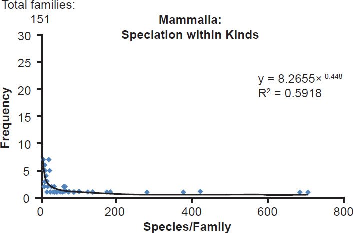
Fig. 1. Power curve distribution of mammalian species per family. The amount of species per family in the class Mammalia was quantified and arrayed in a histogram format. The thin black trendline and equation were derived from the raw data with standard tools in Microsoft Excel.
The same lopsided pattern held true in other vertebrate classes, regardless of whether the class consisted almost entirely of on-Ark kinds (e.g., birds) and or entirely of off-Ark kinds (e.g., bony fish). Reptiles (class Reptilia, Fig. 2), amphibians (class Amphibia, Fig. 3), birds (class Aves, Fig. 4), and bony fish (class Actinopterygii, Fig. 5) all possessed many families with few species and few families with many species (see Supplemental Table 1 for a listing of the common names for many of the taxonomic designations used in this study). Just like the data for the class Mammalia, a power distribution seemed the best approximation for each dataset.
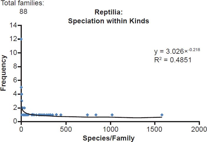
Fig. 2. Power curve distribution of reptile species per family. The amount of species per family in the former class Reptilia was quantified and arrayed in a histogram format. The thin black trendline and equation were derived from the raw data with standard tools in Microsoft Excel.
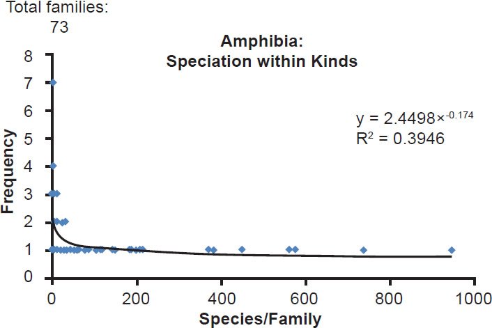
Fig. 3. Power curve distribution of amphibian species per family. The amount of species per family in the class Amphibia was quantified and arrayed in a histogram format. The thin black trendline and equation were derived from the raw data with standard tools in Microsoft Excel.
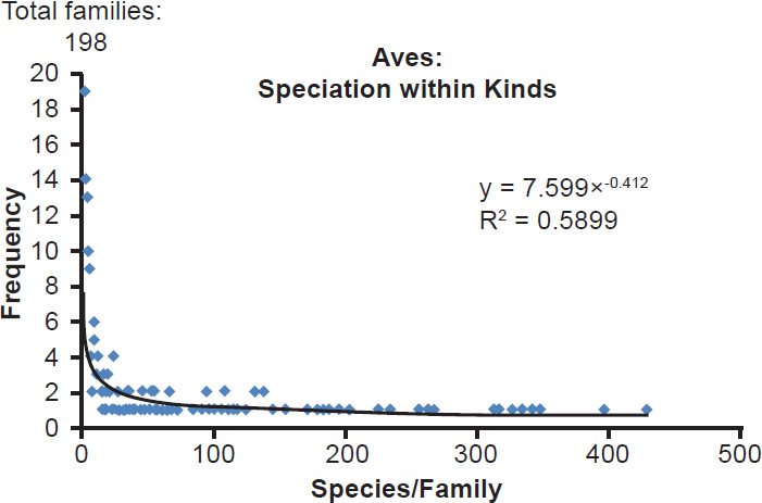
Fig. 4. Power curve distribution of bird species per family. The amount of species per family in the class Aves was quantified and arrayed in a histogram format. The thin black trendline and equation were derived from the raw data with standard tools in Microsoft Excel.
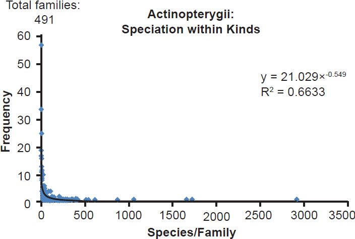
Fig. 5. Power curve distribution of bony fish species per family. The amount of species per family in the class Actinopterygii was quantified and arrayed in a histogram format. The thin black trendline and equation were derived from the raw data with standard tools in Microsoft Excel.
Furthermore, when the species per family counts from all five classes were combined into one dataset, a power distribution matched the data even better. The correlation coefficient for this combined dataset was higher than the coefficient for any of the individual datasets (Fig. 6; Table 1). Overall, the higher the n (number of families) was, the better the fit was to a power law distribution (table 1). Together with Wood’s (2011) results, these data indicate that explosive post-Flood and post-Creation speciation was limited to a select subset of kinds, and it raised the question of whether unusual speciation mechanisms were needed to explain the majority of speciation events in the YE model.
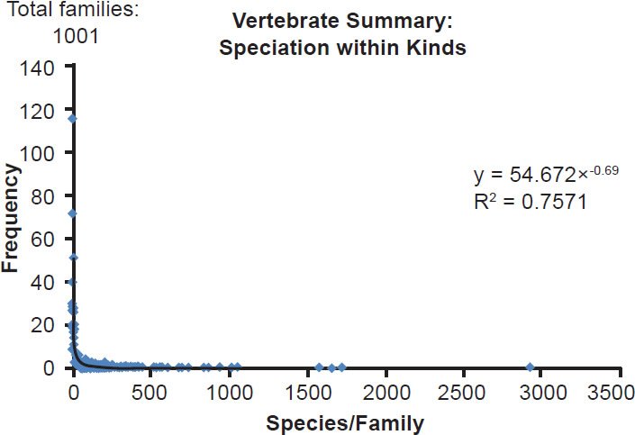
Fig. 6. Power curve distribution of vertebrate species per family. The amount of species per family among the five combined vertebrate classes (Mammalia, Reptilia, Amphibia, Aves, Actinopterygii) was quantified and arrayed in a histogram format. The thin black trendline and equation were derived from the raw data with standard tools in Microsoft Excel.
Table 1. Correlation between number of families and fit to a power curve.
| Group | Total Family # | R2 to Power Curve |
|---|---|---|
| Amphibia | 73 | 0.39 |
| Reptilia | 88 | 0.49 |
| Mammalia | 151 | 0.59 |
| Aves | 198 | 0.59 |
| Actinopterygii | 491 | 0.66 |
| Vertebrates | 1001 | 0.76 |
Assessing the utility of mitochondrial DNA clocks
To investigate the timing of post-Flood and post-Creation speciation, I explored the possibility of using the mitochondrial DNA clock discovered previously (Jeanson 2013). In these previously published results, the amount of mitochondrial DNA diversity matched the expectations of mutation change that had been occurring for 10,000 years or less, and it relied on the mitochondrial DNA sequences published at that time. Since then, more genomes have been published for more species within these groups, and I reinvestigated whether the results would still hold true. Furthermore, since 6000 years and not 10,000 years is generally preferred as the date of creation (Hardy and Carter 2014), I explored whether the results would stand for the more recent date or whether an acceleration in mutation rates was required, as suggested previously (Wood 2012, 2013b).
Like my previous study (Jeanson 2013), I omitted from consideration mitochondrial DNA sequences from fossil or extinct species. Because DNA is such a labile molecule, it seems unlikely that reliable sequences will ever be obtained from samples older than just a few years or decades, unless remarkable care is taken to preserve them. Since the published sequences from extinct species represent samples that have been sitting on or in the ground for hundreds to thousands of years, and for additional reasons following from the discoveries I made below, I left them out of my analyses.
In each of the four extant species or groups of species that I examined, the conclusions from my previously published results (Jeanson 2013) remained the same. For example, in humans, the predicted mitochondrial DNA diversity in the D-loop of non-Africans overlapped the standard deviation in current DNA diversity among non-African ethnic groups (Fig. 7). Also, the predicted mitochondrial DNA diversity in the entire genomes of the three animal groups captured or overlapped existing DNA diversity (Figs. 8–10). Since these four independent data points represented three different phyla as well as both on-Ark and off-Ark creatures, I assumed that mitochondrial DNA clocks existed for the rest of the animal kinds, and I assumed that these clocks “ticked” at a constant rate through time in a manner consistent with the YE timescale.
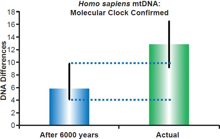
Fig. 7. Human mitochondrial DNA clock. Using the empirically-derived mitochondrial DNA mutation rate for the D-loop in non-African individuals, the predicted amount of DNA differences after 6000 years of mutation at a constant rate was compared to the average D-loop difference among non-African ethnic groups. The height of each colored bar represented the average DNA difference, and the thick black lines represented the 95% confidence interval (“After 6000 years” bar) or standard deviation (“Actual” bar).
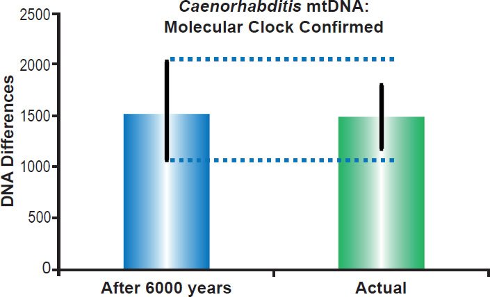
Fig. 8. Roundworm mitochondrial DNA clock. Using the empirically-derived mitochondrial DNA whole genome mutation rate for Caenorhabditis elegans, the predicted amount of DNA differences after 6000 years of mutation at a constant rate was compared to the average difference among Caenorhabditis species. The height of each colored bar represented the average DNA difference, and the thick black lines represented the 95% confidence interval (“After 6000 years” bar) or standard deviation (“Actual” bar).
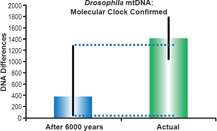
Fig. 9. Fruit fly mitochondrial DNA clock. Using the empirically-derived mitochondrial DNA whole genome mutation rate for Drosophila melanogaster, the predicted amount of DNA differences after 6000 years of mutation at a constant rate was compared to the average difference among Drosophila species. The height of each colored bar represented the average DNA difference, and the thick black lines represented the 95% confidence interval (“After 6000 years” bar) or standard deviation (“Actual” bar).
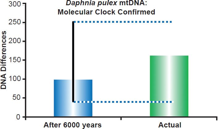
Fig. 10. Water flea mitochondrial DNA clock. Using the empirically-derived mitochondrial DNA whole genome mutation rate for Daphnia pulex, the predicted amount of DNA differences after 6000 years of mutation at a constant rate was compared to the maximum difference between Daphnia pulex individuals. The height of each colored bar represented the average (predicted) or maximum (actual) DNA difference, and the thick black line represented the 95% confidence interval.
To date, no further mitochondrial DNA mutation rates have been measured in additional animal species. Nevertheless, for those species with a published mitochondrial DNA whole genome sequence, comparative DNA analysis was still possible, and the resultant patterns might be informative. Hence, I proceeded to interrogate the question of the timing of speciation by restricting my investigation to analysis of comparative mitochondrial DNA sequence patterns under a set of simplifying assumptions.
First, in addition to assuming that a mitochondrial DNA clock exists for each “kind” and that the mitochondrial DNA mutation rate was constant through time, I assumed that the mitochondrial DNA mutation rate was constant across lineages.
This assumption was partially testable based on the presence or absence of signature patterns in the mitochondrial DNA trees for the kinds I investigated. These signature patterns derived from an analysis of the human mitochondrial DNA tree for the various ethnic groups and from an analysis of the text of Genesis. According to Genesis 9:18–19, “Now the sons of Noah who went out of the ark were Shem, Ham, and Japheth. And Ham was the father of Canaan. These three were the sons of Noah, and from these the whole earth was populated” (NKJV). Thus, since there are more than three different ethnic groups in existence today, our modern ethnic groups must have arisen post-Flood, likely as a result of the confusion of languages at Babel (Genesis 11).
Furthermore, this history would likely have been recorded in the mitochondrial DNA patterns around the world. Since mitochondrial DNA is inherited maternally, the fact of the Flood and the fact of the tower of Babel led to very specific expectations about the comparative DNA patterns observable today. Because four women survived the Flood, no more than four major ancestral mitochondrial DNA lineages could have given rise to the modern ethnic groups. In fact, no more than three should have been present (Carter 2010). Though Noah’s wife passed on her mitochondrial DNA to her three sons, her lineage then ceased since men do not pass on their mitochondrial DNA to their offspring. Instead, all modern mitochondrial DNA lineages should trace back to the three wives of Noah’s sons.
Remarkably, upon visual inspection of the human mitochondrial DNA tree of various modern ethnic groups, three nodes were visually apparent (Figs. 11A–B). In addition, most of the ethnic lineages stemming from these three nodes sprayed out almost immediately rather than staggering out (Fig. 11A), as if they arose from a divergence event rather than a coalescence event, a finding consistent with the description and timing of the Tower of Babel incident in Genesis 11.
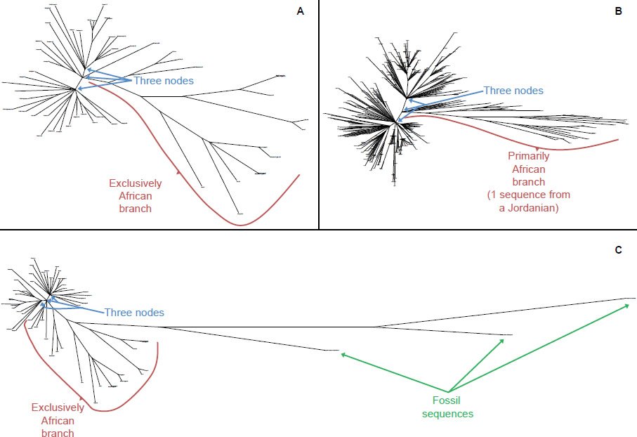
Fig. 11. Three-node structure of the human mitochondrial DNA tree. A Whole genome alignment and resultant phylogenetic tree of 53 human ethnic groups. Upon visual inspection, three major subgroups or nodes were visible. One of the nodes was exclusively African lineages, and some of the branches stemming from this node were about twice as long as the other branches. B Whole genome alignment and resultant phylogenetic tree of 371 human individuals from various human ethnic groups. Similar to A, visual inspection demonstrated the existence of three major subgroups or nodes. Again, like A one of the nodes was almost exclusively African lineages, and some of the branches stemming from this node were about twice as long as the other branches. C Same data as A but with three fossil human sequences included. Similar to A visual inspection demonstrated the existence of three major subgroups or nodes. Again, like A one of the nodes was exclusively African lineages, and some of the branches stemming from this node were about twice as long as the other branches. Surprisingly, all three fossil human individuals branched off from the exclusively African lineage, and their branch lengths were much longer than those of the extant human individuals.
This fact of the three nodes in the human mitochondrial DNA tree had ramifications for the constancy of the rates of genetic change across lineages. If the three nodes did indeed represent the sequences in the wives of Noah’s sons, then those nodes represented an identical point in time, which means that all their descendants had been mutating for an identical length of time. For non-Africans lineages (e.g., two of the three major nodes in the tree), the current and empirically measured rate of change in the D-loop matches the predictions of the hypothesis that the rate of change has been constant with time (Fig. 7).
By contrast, the section of the tree containing exclusively African lineages had a maximum branch length about twice as long as the non-African branches (Fig. 11). Presumably, some of the lineages in the African branch had been mutating twice as fast as the non-African branches, giving rise to the discrepancy in branch lengths. This hypothesis had preliminary support in the discovery that another form of genetic change, recombination, occurs faster in African than in non-Africans (Hinch et al. 2011). Together, these facts suggested that visual examination of radiation style trees with visually obvious roots might identify lineages with faster or slower rates than the overall rate. Hence, before performing species’ time of origin analyses within animal families, I created a radiation style tree for each family, visually inspected the trees for obvious roots, and visually compared the branch lengths about the proposed root to assess the possibility of rate heterogeneity across species within a family (Supplemental Figs. 1–24, 49–51).
The branch length patterns among the three nodes in the human tree lent further support to the exclusion of fossil sequences from consideration in the present analyses. When the Homo heidelbergensis, Homo sp. Altai, and Homo sapiens neanderthalensis mitochondrial genomes were included in the analysis, two facts were immediately apparent. First, these sequences were indeed quite divergent from the mitochondrial DNA sequences of extant human ethnic groups (Fig. 11C). Second, all three fossil sequences branched off from the exclusively African lineage (Fig. 11C). This suggested that, if the fossil sequences were indeed reliable, they represented a subsection of the African lineage with an unusually high mutation rate. In fact, the high rate may have caused the extinction of these ancient human populations. Alternatively, these sequences may still be degraded. Regardless of which of these two explanations was true, fossil sequences clearly represented an unusual set of data, and these data did not contradict the assumption in modern lineages of constant rates of mitochondrial DNA mutation through time.
Since these results implied that the three nodes represented the sequences of the three wives of Noah’s sons, the data further implied that the sequence of mitochondrial “Eve” was located somewhere between them. Previous YE creationist studies (Carter, Criswell, and Sanford 2008) of mitochondrial “Eve” placed her sequence, not between these three nodes, but exactly centered on one of them (Fig. 12). This finding may have been an artifact of the methodology used, a possibility the authors readily acknowledged. Since Carter, Criswell, and Sanford inferred the “Eve” sequence from the majority allele at each position in the mitochondrial genome, and since the node upon which “Eve” is centered represents three-fourths of the sequence samples, the parameters of their methods almost guaranteed that Eve would land exactly at the node most represented. Alternatively, since so few generations passed between Adam and Noah according to Genesis 5, one of the wives of Noah’s sons may have inherited her DNA sequence with little to no mutations from Eve’s original created sequence. Regardless of the explanation, the results and inferences of the present study were reconcilable with previously published YE creationist data on mitochondrial “Eve.”
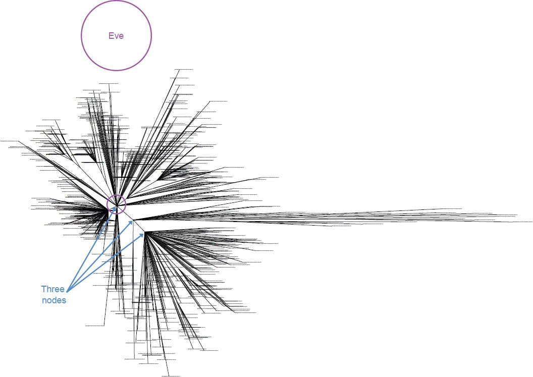
Fig. 12. Location of mitochondrial “Eve” within the three-node structure of the human mitochondrial DNA tree. Whole genome alignment and resultant phylogenetic tree of 828 human individuals plus the previously derived mitochondrial “Eve” sequence. Similar to Fig. 11, three major nodes were visible, and “Eve” was located at one of the nodes which happened to be the node containing the most individuals in the dataset.
Speciation rate analyses required a second assumption besides the assumption of rate homogeneity. Since species have formed post-Creation and post-Flood, there obviously existed a point in time when speciation commenced. Since we currently lack measured mitochondrial DNA mutation rates for the vast majority of animal families, absolute rooting of each family’s mitochondrial DNA tree was impossible at present.
However, the majority of families appeared to pass the visual rate homogeneity test (Supplemental Figs. 1–24, 49–51). Twenty-four of the families all displayed an easily identifiable root from which species radiated with roughly equal branch lengths (Supplemental Figs. 1, 3–12, 14, 16–24). Only Ursidae (Supplemental Fig. 2), Gruidae (Supplemental Fig. 13), and Crocodylidae (Supplemental Fig. 15) had radiation style trees resembling the human mitochondrial DNA tree. These three animal families had visually identifiable roots from which most species in the family had roughly equivalent branch lengths, but from which a few species had unusually long branch lengths. Thus, for most of the families, rooting the tree on the midpoint seemed a reasonable approximation of the start of the speciation process.
Furthermore, mitochondrial DNA sequence alignments above the taxonomic rank of family indicated that, between some families, relatively few DNA differences existed (Fig. 13). If large numbers of DNA differences had separated families, this fact would have raised concerns that mutations had been ongoing long before speciation commenced. Since relatively few DNA differences separated unrelated (i.e., separately created) families, the assumption that the midpoint approximated the start of the speciation process gained further credibility.
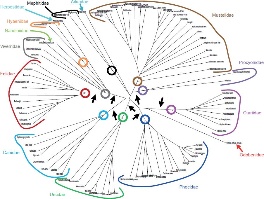
Fig. 13. Mitochondrial DNA differences among species within Carnivora. Whole genome alignment and resultant DNA differences depicted as branch lengths on a tree. Species within a family were highlighted with different colors. Colored circles represented the deepest root for each family. As the black arrows highlighted, the DNA differences separating the roots of different families were short relative to the DNA differences separating the species within a family.
Hence, for each family I created linearized trees, rooted the trees on the midpoint, and assumed that speciation began at the midpoint (Supplemental Figs. 25–48, 52–53). For on-Ark “kinds,” I assumed that the midpoint represented the first year immediately post-Flood (e.g., 4350 years ago). For off-Ark “kinds,” I assumed that the midpoint represented the first year immediately post-Creation (e.g., 6000 years ago). If some “kinds” did not form a single new species until late post-Creation or late post-Flood, this methodology would miss this fact. However, since rapid speciation early post-Flood was the prevailing hypothesis, I effectively set up this experiment to be overly generous towards the early speciation view.
I also made a third assumption in these genetic analyses, namely, that the branch point between two species represented the actual speciation event. This hypothesis was partially tested by aligning the sequences from multiple individuals within each species. For the families Bovidae, Ursidae, and Hominidae, species existed for which sequences from multiple individuals were present in the NCBI databases. If branch points on the tree did not represent speciation events, then this analysis should have resulted in crossing and mixing up of the branches from multiple individuals in separate species. In other words, there should have been no obvious single branch point separating all the individuals within a species from all the other individuals in a separate species.
After aligning sequences from individuals within each of these families and then drawing trees reflecting only the topology of the relationships, a single branch point still separated species from one another. No overlapping branches were found, and no branches from separate species crossed (Figs. 14–16). Thus, the assumption that the branch point represents a speciation event seemed reasonable.
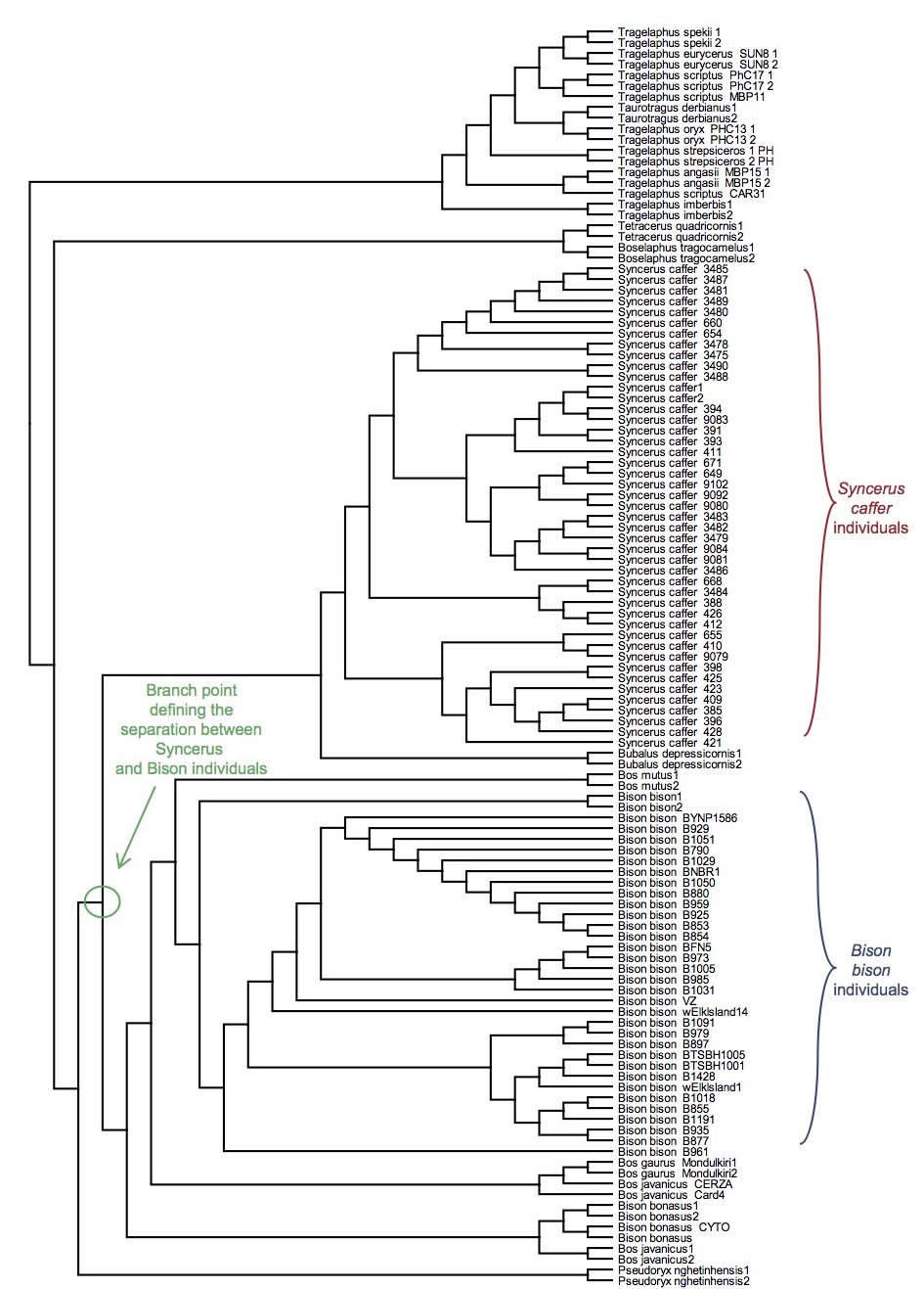
Fig. 14. Topology-only tree of Bovinae individuals and species. Whole genome alignment and resultant branching relationships depicted in a topology-only diagram. Lengths of the branches did not correspond exactly to actual DNA differences but did depict branching relationships. As was apparent upon visual inspection, neither the Syncerus caffer individuals nor the Bison bison individuals ever had branches intermixed with branches from other species, consistent with the hypothesis that branch points correspond to actual speciation events.
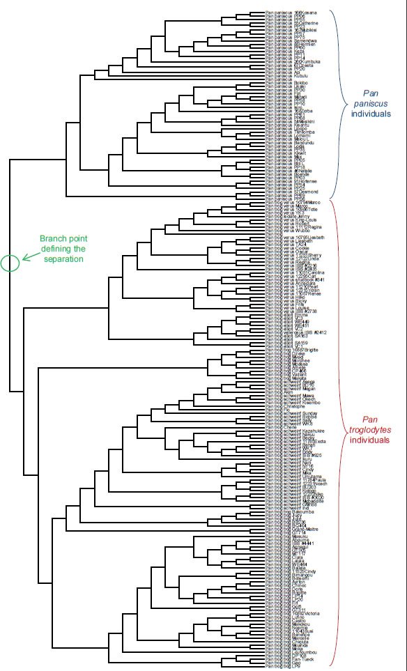
Fig. 15. Topology-only tree of Pan individuals and species. Whole genome alignment and resultant branching relationships depicted in a topology-only diagram. Lengths of the branches did not correspond exactly to actual DNA differences but did depict branching relationships. As was apparent upon visual inspection, none of the individuals within Pan paniscus and Pan troglodytes ever had branches intermixed with branches from the other species, consistent with the hypothesis that branch points correspond to actual speciation events.
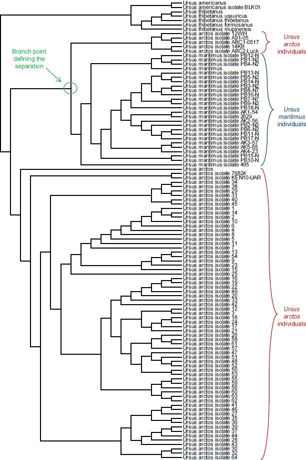
Fig. 16. Topology-only tree of Ursus individuals and species. Whole genome alignment and resultant branching relationships depicted in a topology-only diagram. Lengths of the branches did not correspond exactly to actual DNA differences but did depict branching relationships. As was apparent upon visual inspection, neither the Ursus arctos individuals nor the Ursus maritimus individuals ever had branches intermixed with branches from other species, consistent with the hypothesis that branch points correspond to actual speciation events. Though the Ursus arctos individuals appeared to stem from two different populations, the individuals from Ursus maritimus were still clearly distinct from Ursus arctos individuals.
Conversely, when a tree was drawn to reflect the actual DNA differences rather than just the topology of the relationships, the branch lengths appeared to reflect recent historical events. From recorded history, the American bison (Bison bison) and African buffalo (Syncerus caffer) appear to have undergone population bottlenecks of different sizes. From population estimates of millions to tens of millions of individuals worldwide, the American bison was hunted to less than 1000 individuals globally in the late 1800s/early 1900s—a >99.9% reduction in population size (Gates et al. 2010). Currently, the numbers have recovered to only ~530,000 individuals (Gates and Aune 2008). By contrast, the African buffalo population lost only 80–90% of its individuals (Mack 1970) in the late 1800s, and its current worldwide population size is closer to 1,000,000 than 500,000 (IUCN SSC Antelope Specialist Group 2008).
Since the mitochondrial DNA branch lengths reflect the time to a common ancestor, and since this time is a function of effective population size (Futuyma 2009), population genetics would predict a shorter coalescence time (branch length) for the American bison population than for the African buffalo population. In fact, actual branch lengths matched this prediction (Fig. 17). Hence, branch lengths appeared to record real historical events within species.
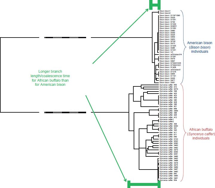
Fig. 17. Different coalescent times within Bovinae. Whole genome alignment and resultant DNA differences depicted as branch lengths on a tree. To magnify the differences in branch lengths among Syncerus caffer and Bison bison individuals, the middle section of the tree was omitted, as indicated by the dashed lines. Upon visual inspection, it was apparent that the branch lengths connecting the most distant Syncerus caffer individuals were longer than the branch lengths connecting the most distant Bison bison individuals. Hence, the coalescence time for Syncerus caffer was longer than for Bison bison, consistent with the recent and more dramatic population bottleneck experienced by Bison bison.
Given this precedence within species, it seemed plausible to assume that branch points represented or at least approximated real speciation events between species. Though multiple individuals may have been part of the speciation event itself, and though the actual event may have been slightly before or after the time represented by the branch point, using the branch point as a surrogate for the time of speciation appeared to be a reasonable first approximation.
Speciation hypotheses
With these methodological parameters in mind, I derived several expectations in light of the prevailing YE hypotheses on the timing of speciation. These hypotheses and their predictions can be divided into four general categories. As Wise (1994) and Wood (2002, 2003) have previously speculated, speciation post-Flood and even post-Creation may have been early and rapid followed by a long period of little speciation (the “Early episode” hypothesis, Fig. 18). Alternatively, it is possible that this timeline was flipped—a long period of little speciation followed by a rapid burst in the recent past (the “Late” hypothesis, Fig. 18). As Wise (1994) and Wood (2002, 2003) have pointed out previously, this hypothesis seems unlikely since recent history records hardly any speciation events. Nonetheless, it was worth testing. Finally, speciation may have occurred at a constant rate (“Linear,” Fig. 18), or it may have involved a series of bursts (“Episodic,” Fig. 18).
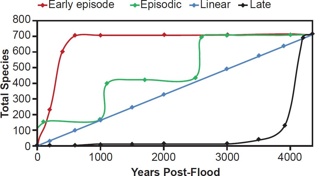
Fig. 18. Hypotheses on the timing of speciation within biblical parameters. Using the family Muridae (712 total species) as an example of a speciose family, contrasting hypotheses on the timing of speciation post-Flood were depicted visually. The “Early episode” hypothesis represented one in which speciation happened in a rapid burst and then quickly tapered off. The “Episodic” hypothesis represented a proposal that speciation happened in several short bursts over time. The “Linear” hypothesis represented a guess that the speciation rate has been constant with time, while the “Late” hypothesis represented the mirror image of the “Early episode”—that speciation rates were virtually zero for several thousand years and then recently and rapidly increased to high levels.
Genetic patterns fit the linear speciation hypothesis
I tested these four hypotheses by aligning the mitochondrial DNA sequences for species within a family, creating a tree to reflect the DNA differences, and then linearizing the tree and rooting it on the midpoint, as per the assumptions I articulated above. I then used the branch lengths between each branch point as a surrogate for time between speciation events and created a timeline from these DNA differences.
These analyses were limited by the fact that not all species within a family were represented by DNA sequences in the curated public databases. For example, among the most speciose mammal families (e.g., those with 60 or more species), only the family Bovidae had 75% of its species represented in the NCBI RefSeq database (Table 2). The remainder of these speciose families lacked 50% species representation, and most lacked even 10% species representation (Table 2).
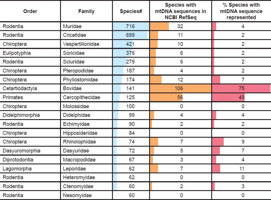
Table 2. Mammalian species representation per family in NCBI RefSeq database.
Nevertheless, in the family Bovidae, the pattern of speciation was abundantly clear. The trajectory of speciation was a very tight fit (R2 = 0.997) with the linear speciation hypothesis (Fig. 19). In addition, since 48 of 52 (92%) genera within Bovidae were represented in these data, eventual publication of the mitochondrial DNA sequences from the remaining species within Bovidae seemed unlikely to change the match between linear speciation hypothesis and the actual speciation timeline.
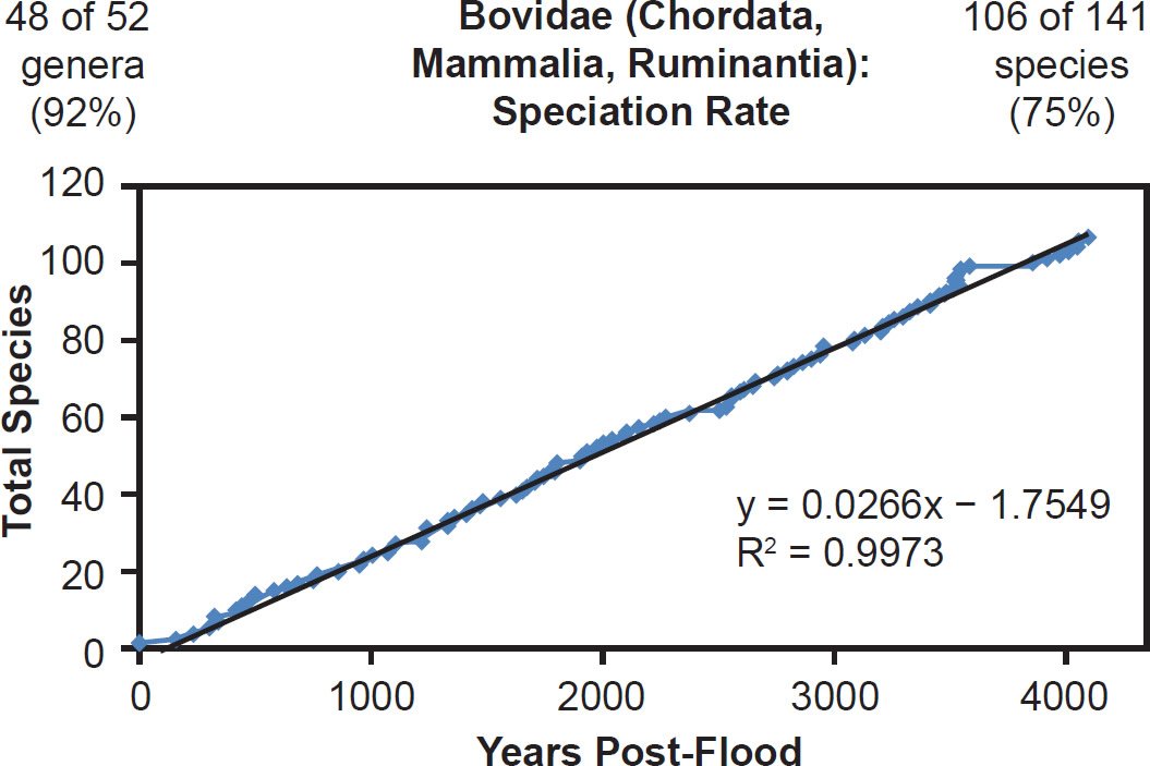
Fig. 19. Speciation rate within the family Bovidae. Whole genome alignments for extant, wild (non-domestic) species in the family Bovidae were performed. A phylogenetic tree was created from which branch lengths between branch points were extracted, converted to years, and used to plot the timeline of branching/ speciation within the family. The results were a tight fit to a linear function, which was represented by the thin black line and the equation, both of which were derived via linear regression of the raw data in Microsoft Excel. Representation of genera and species within the family were depicted in the upper left and right corners, respectively.
I also assessed several mammal families whose species were completely represented in the NCBI RefSeq database. Though several families with four or fewer species were completely represented, under the assumptions I made for these analyses, tree-drawing and curve-fitting for these families would have been statistically uninformative. For mammals, this effectively eliminated 38% (58 of 151) of the families from consideration. Of the remaining 62%, three were fully represented in the NCBI RefSeq database: Ursidae, Rhinocerotidae, and Balaenopteridae. All three of these families fit the linear speciation rate hypothesis (Figs. 20–22).
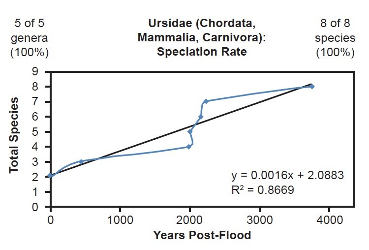
Fig. 20. Speciation rate within the family Ursidae. Whole genome alignments for extant species in the family Ursidae were performed. A phylogenetic tree was created from which branch lengths between branch points were extracted, converted to years, and used to plot the timeline of branching/speciation within the family. The results were a good fit to a linear function, which was represented by the thin black line and the equation, both of which were derived via linear regression of the raw data in Microsoft Excel. Representation of genera and species within the family were depicted in the upper left and right corners, respectively.
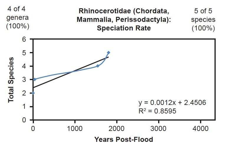
Fig. 21. Speciation rate within the family Rhinocerotidae. Whole genome alignments for extant species in the family Rhinocerotidae were performed. A phylogenetic tree was created from which branch lengths between branch points were extracted, converted to years, and used to plot the timeline of branching/speciation within the family. The results were a good fit to a linear function, which was represented by the thin black line and the equation, both of which were derived via linear regression of the raw data in Microsoft Excel. Representation of genera and species within the family were depicted in the upper left and right corners, respectively.
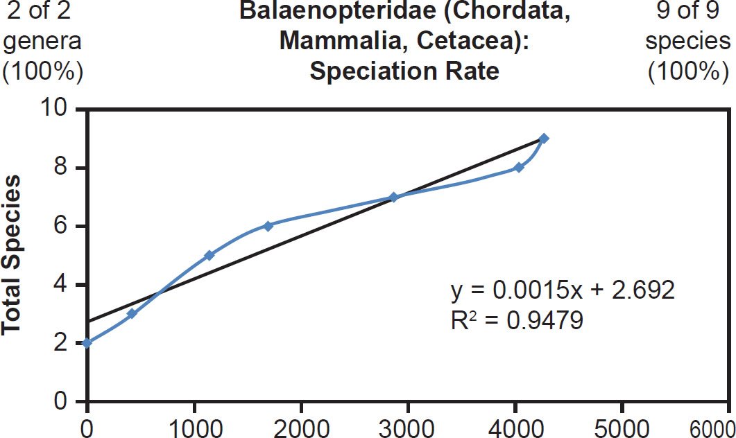
Fig. 22. Speciation rate within the family Balaenopteridae. Whole genome alignments for extant species in the family Balaenopteridae were performed. A phylogenetic tree was created from which branch lengths between branch points were extracted, converted to years, and used to plot the timeline of branching/ speciation within the family. The results were a fairly tight fit to a linear function, which was represented by the thin black line and the equation, both of which were derived via linear regression of the raw data in Microsoft Excel. Representation of genera and species within the family were depicted in the upper left and right corners, respectively.
Though the correlation coefficient for each of these families was lower than the coefficient for the Bovidae family, this result may have been an artifact of small number statistics. Since Ursidae, Rhinocerotidae, and Balaenopteridae had only eight, five, and nine species total, respectively, small deviations from the mean would have had higher statistical consequence than deviations in a family with over 100 data points. Furthermore, since the radiation style tree for Ursidae suggested the possibility of different rates of change for at least two of the Ursid species (Supplemental Fig. 2), the lower correlation coefficient may have been a consequence of non-identical mutation rates across species within the Ursidae family. Hence, these data from three on-Ark families (Bovidae, Ursidae, Rhinocerotidae) and one off-Ark family (Balaenopteridae) all depicted the same result: A linear timeline of speciation.
For mammal families with incomplete species representation in the NCBI RefSeq database but higher representation than Bovidae, a match between the linear speciation rate hypothesis and the data was the rule. Equidae (Fig. 23), Hominidae (Fig. 24), and Phocidae (Fig. 25) all fit the linear rate hypothesis well.
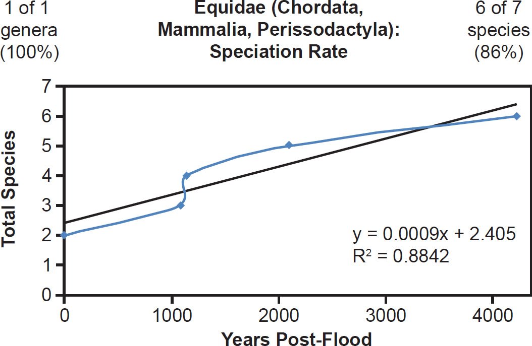
Fig. 23. Speciation rate within the family Equidae. Whole genome alignments for extant, wild (non-domestic) species in the family Equidae were performed. A phylogenetic tree was created from which branch lengths between branch points were extracted, converted to years, and used to plot the timeline of branching/ speciation within the family. The results were a good fit to a linear function, which was represented by the thin black line and the equation, both of which were derived via linear regression of the raw data in Microsoft Excel. Representation of genera and species within the family were depicted in the upper left and right corners, respectively.
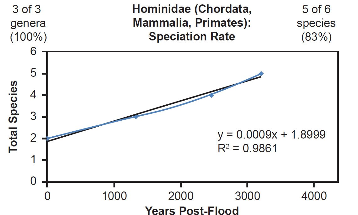
Fig. 24. Speciation rate within the family Hominidae. Whole genome alignments for extant species in the family Hominidae were performed. A phylogenetic tree was created from which branch lengths between branch points were extracted, converted to years, and used to plot the timeline of branching/speciation within the family. The results were a tight fit to a linear function, which was represented by the thin black line and the equation, both of which were derived via linear regression of the raw data in Microsoft Excel. Representation of genera and species within the family were depicted in the upper left and right corners, respectively.
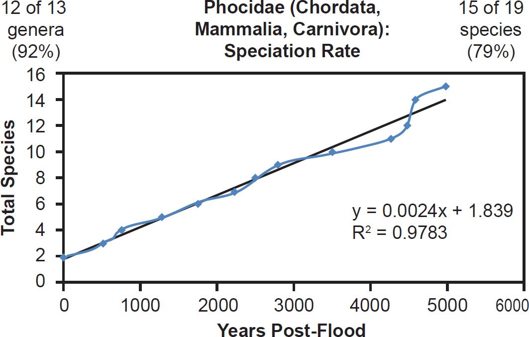
Fig. 25. Speciation rate within the family Phocidae. Whole genome alignments for extant species in the family Phocidae were performed. A phylogenetic tree was created from which branch lengths between branch points were extracted, converted to years, and used to plot the timeline of branching/speciation within the family. The results were a tight fit to a linear function, which was represented by the thin black line and the equation, both of which were derived via linear regression of the raw data in Microsoft Excel. Representation of genera and species within the family were depicted in the upper left and right corners, respectively.
Even mammal families that were moderately to intensely speciose but less well-represented with mitochondrial DNA sequences displayed a linear pattern. Cervidae (61% species representation, Fig. 26), Cercopithecidae (45% species representation, Fig. 27), Mustelidae (42% species representation, Fig. 28), Delphinidae (49% species representation, Fig. 29), and even Muridae (4% species representation, Fig. 30) all fit a linear speciation rate with little to any evidence of a burst of speciation immediately post-Flood or post-Creation. Thus, independent of Ark status (e.g., on- or off-Ark), mammalian order (e.g., Ruminantia, Carnivora, Perissodactyla, Cetacea, Primates, and Rodentia), and species DNA sequence representation (e.g., 100% to 4%), mammal families showed a linear rate of speciation since the Flood or since Creation (Figs. 19–30).
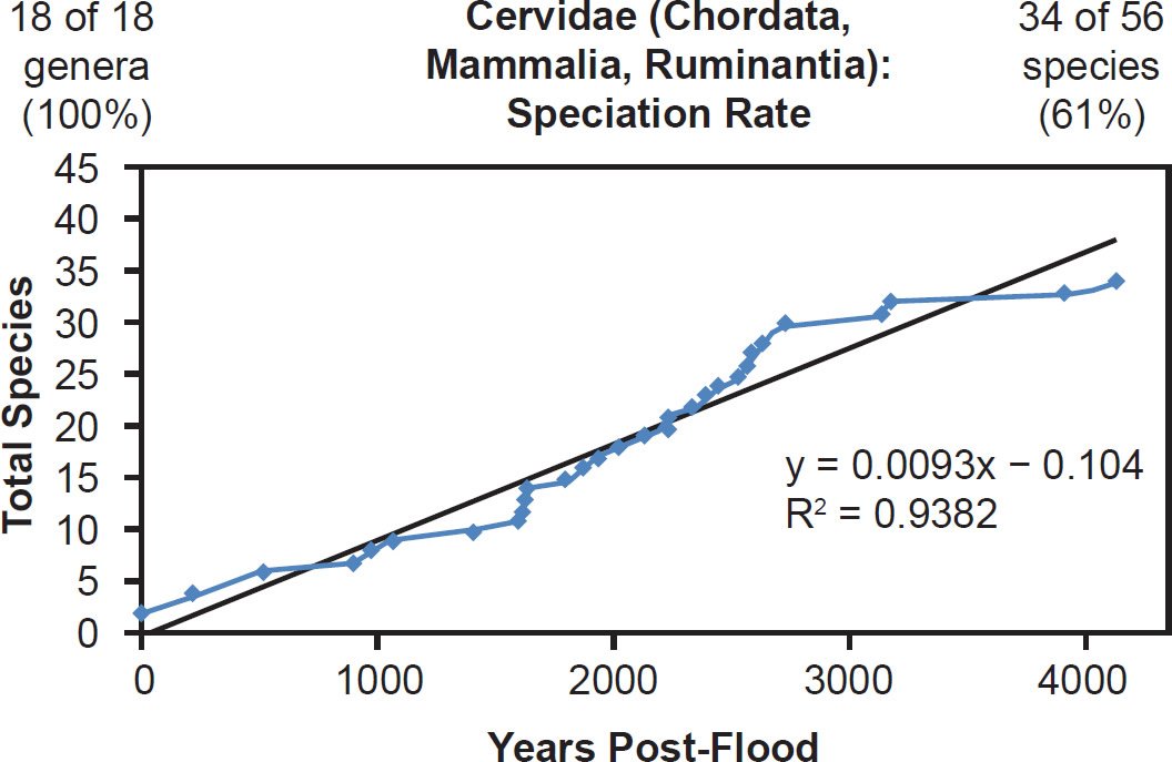
Fig. 26. Speciation rate within the family Cervidae. Whole genome alignments for extant species in the family Cervidae were performed. A phylogenetic tree was created from which branch lengths between branch points were extracted, converted to years, and used to plot the timeline of branching/speciation within the family. The results were a fairly tight fit to a linear function, which was represented by the thin black line and the equation, both of which were derived via linear regression of the raw data in Microsoft Excel. Representation of genera and species within the family were depicted in the upper left and right corners, respectively.
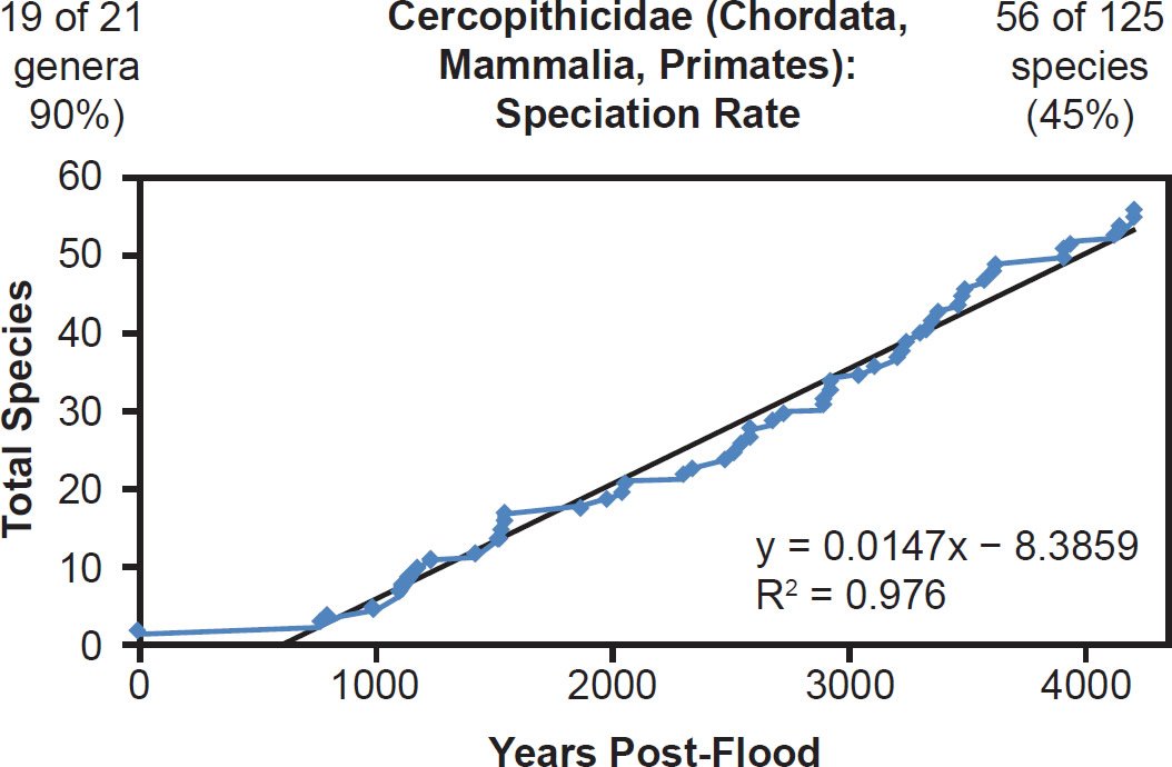
Fig. 27. Speciation rate within the family Cercopithecidae. Whole genome alignments for extant species in the family Cercopithecidae were performed. A phylogenetic tree was created from which branch lengths between branch points were extracted, converted to years, and used to plot the timeline of branching/speciation within the family. The results were a tight fit to a linear function, which was represented by the thin black line and the equation, both of which were derived via linear regression of the raw data in Microsoft Excel. Representation of genera and species within the family were depicted in the upper left and right corners, respectively.
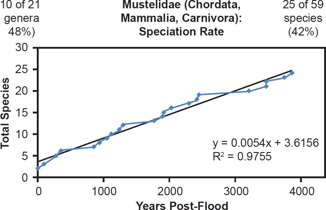
Fig. 28. Speciation rate within the family Mustelidae. Whole genome alignments for extant species in the family Mustelidae were performed. A phylogenetic tree was created from which branch lengths between branch points were extracted, converted to years, and used to plot the timeline of branching/speciation within the family. The results were a tight fit to a linear function, which was represented by the thin black line and the equation, both of which were derived via linear regression of the raw data in Microsoft Excel. Representation of genera and species within the family were depicted in the upper left and right corners, respectively.
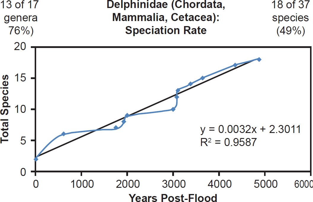
Fig. 29. Speciation rate within the family Delphinidae. Whole genome alignments for extant species in the family Delphinidae were performed. A phylogenetic tree was created from which branch lengths between branch points were extracted, converted to years, and used to plot the timeline of branching/speciation within the family. The results were a fairly tight fit to a linear function, which was represented by the thin black line and the equation, both of which were derived via linear regression of the raw data in Microsoft Excel. Representation of genera and species within the family were depicted in the upper left and right corners, respectively.
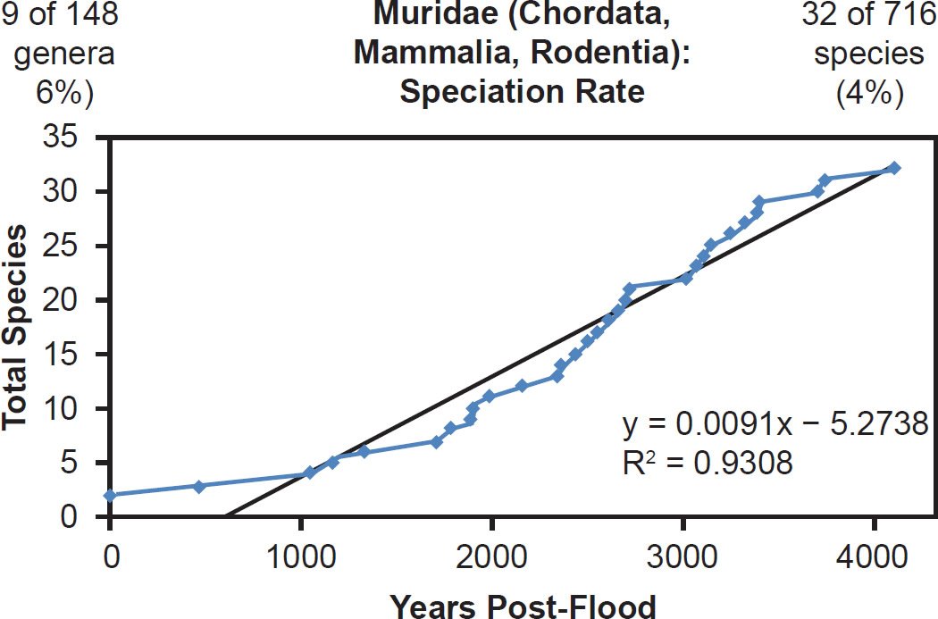
Fig. 30. Speciation rate within the family Muridae. Whole genome alignments for extant species in the family Muridae were performed. A phylogenetic tree was created from which branch lengths between branch points were extracted, converted to years, and used to plot the timeline of branching/speciation within the family. The results were a fairly tight fit to a linear function, which was represented by the thin black line and the equation, both of which were derived via linear regression of the raw data in Microsoft Excel. Representation of genera and species within the family were depicted in the upper left and right corners, respectively.
This linear pattern was true across vertebrate classes. Within Aves, both well-represented (Gruidae, 100% species representation, Fig. 31) and poorly represented (Phasianidae, 26% species representation, Fig. 32) families generally matched the linear speciation rate hypothesis. As per the visual rate homogeneity test (Supplemental Fig. 13), lineages within Gruidae may have undergone unequal rates of mutation change. Hence, if this unequal mutation rate hypothesis was indeed true, then the correlation coefficient for Gruidae might have been even higher had mutation rates been identical across lineages.
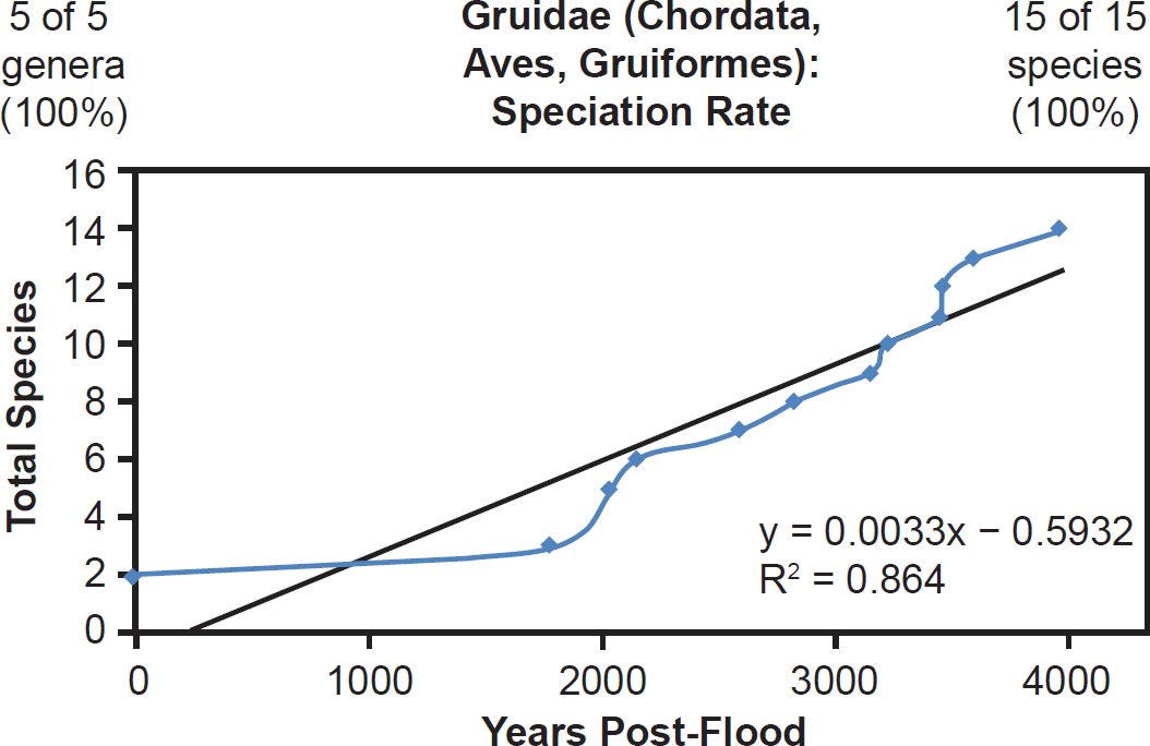
Fig. 31. Speciation rate within the family Gruidae. Whole genome alignments for extant species in the family Gruidae were performed. A phylogenetic tree was created from which branch lengths between branch points were extracted, converted to years, and used to plot the timeline of branching/speciation within the family. The results were a good fit to a linear function, which was represented by the thin black line and the equation, both of which were derived via linear regression of the raw data in Microsoft Excel. Representation of genera and species within the family were depicted in the upper left and right corners, respectively.
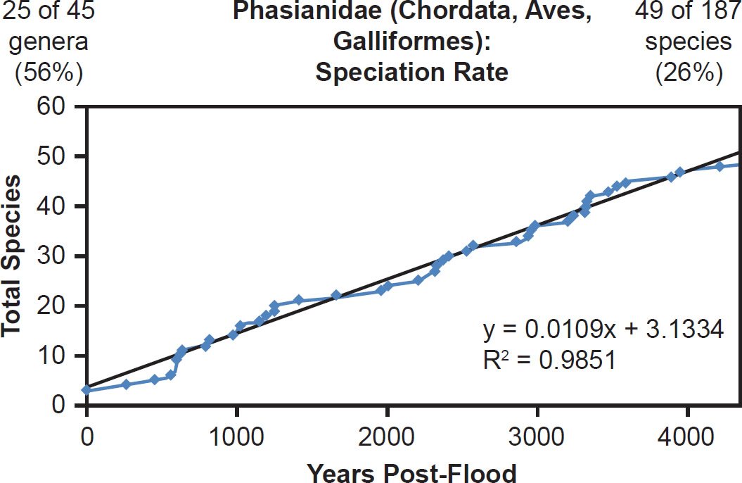
Fig. 32. Speciation rate within the family Phasianidae. Whole genome alignments for extant species in the family Phasianidae were performed. A phylogenetic tree was created from which branch lengths between branch points were extracted, converted to years, and used to plot the timeline of branching/speciation within the family. The results were a tight fit to a linear function, which was represented by the thin black line and the equation, both of which were derived via linear regression of the raw data in Microsoft Excel. Representation of genera and species within the family were depicted in the upper left and right corners, respectively.
In addition, some of the best-represented reptile (Crocodylidae, 81% species representation, Fig. 33) and amphibian (Hynobiidae, 42% species representation, Fig. 34) families also matched the linear speciation hypothesis. Again, the visual rate homogeneity test for Crocodylidae suggested that mutation rates were unequal across lineages within the family (Supplemental Fig. 15). Thus, if this unequal mutation rate hypothesis was indeed true, the correlation coefficient for Crocodylidae might have been even higher had rates been identical across lineages. Regardless, the existing results still matched the linear speciation rate hypothesis.
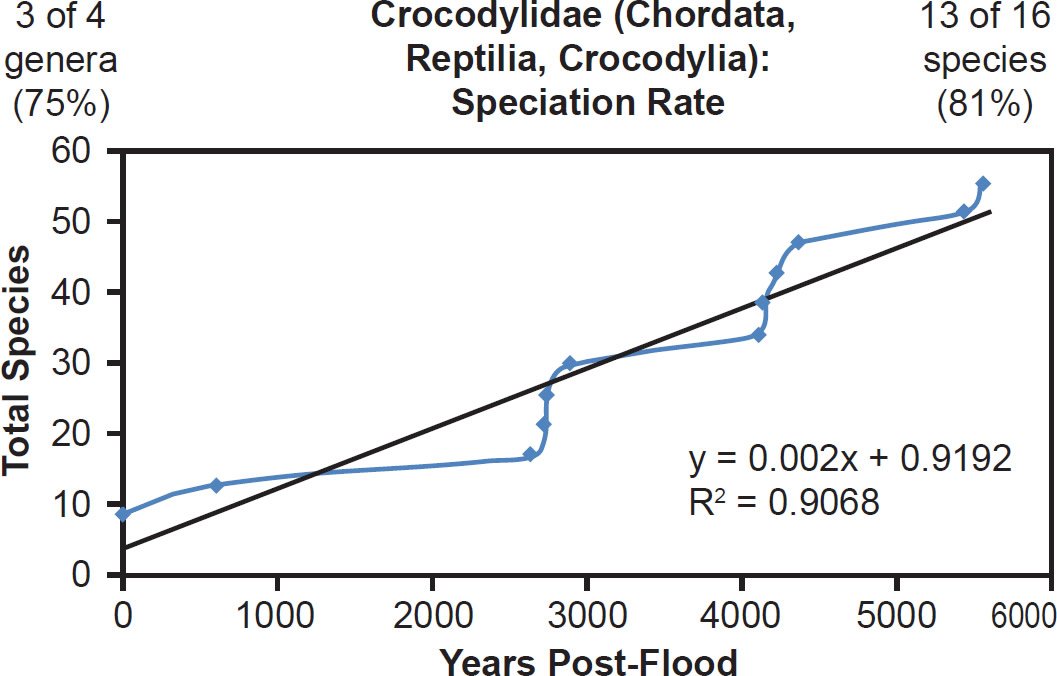
Fig. 33. Speciation rate within the family Crocodylidae. Whole genome alignments for extant species in the family Crocodylidae were performed. A phylogenetic tree was created from which branch lengths between branch points were extracted, converted to years, and used to plot the timeline of branching/speciation within the family. The results were a good fit to a linear function, which was represented by the thin black line and the equation, both of which were derived via linear regression of the raw data in Microsoft Excel. Representation of genera and species within the family were depicted in the upper left and right corners, respectively.
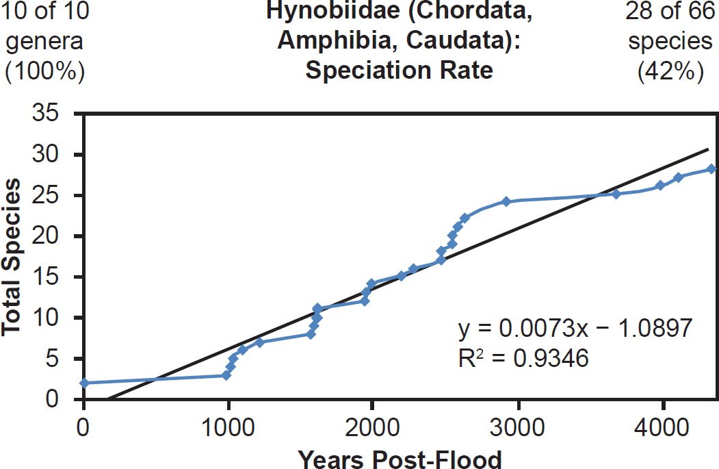
Fig. 34. Speciation rate within the family Hynobiidae. Whole genome alignments for extant species in the family Hynobiidae were performed. A phylogenetic tree was created from which branch lengths between branch points were extracted, converted to years, and used to plot the timeline of branching/speciation within the family. The results were a fairly tight fit to a linear function, which was represented by the thin black line and the equation, both of which were derived via linear regression of the raw data in Microsoft Excel. Representation of genera and species within the family were depicted in the upper left and right corners, respectively.
Among fish families, whether the species representation by DNA sequences was high (Anguillidae, 89%), intermediate (Scombridae, 47%), or low (Tetraodontidae, 31%), linear rates of speciation were the rule (Figs. 35–37). Even the most species-rich family across all vertebrate classes (Cyprinidae, 2935 extant species) showed a strongly linear speciation rate, despite having only 10% of its species represented by mitochondrial DNA sequences (Fig. 38). Thus, linear rates were independent of Ark status, species representation, and mammalian order, and they were also independent of vertebrate class.
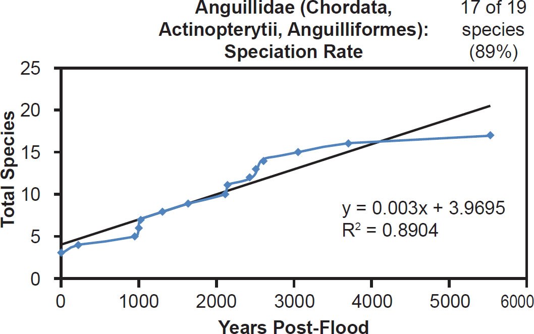
Fig. 35. Speciation rate within the family Anguillidae. Whole genome alignments for extant species in the family Anguillidae were performed. A phylogenetic tree was created from which branch lengths between branch points were extracted, converted to years, and used to plot the timeline of branching/speciation within the family. The results were a good fit to a linear function, which was represented by the thin black line and the equation, both of which were derived via linear regression of the raw data in Microsoft Excel. Representation of species within the family was depicted in the upper right corner.
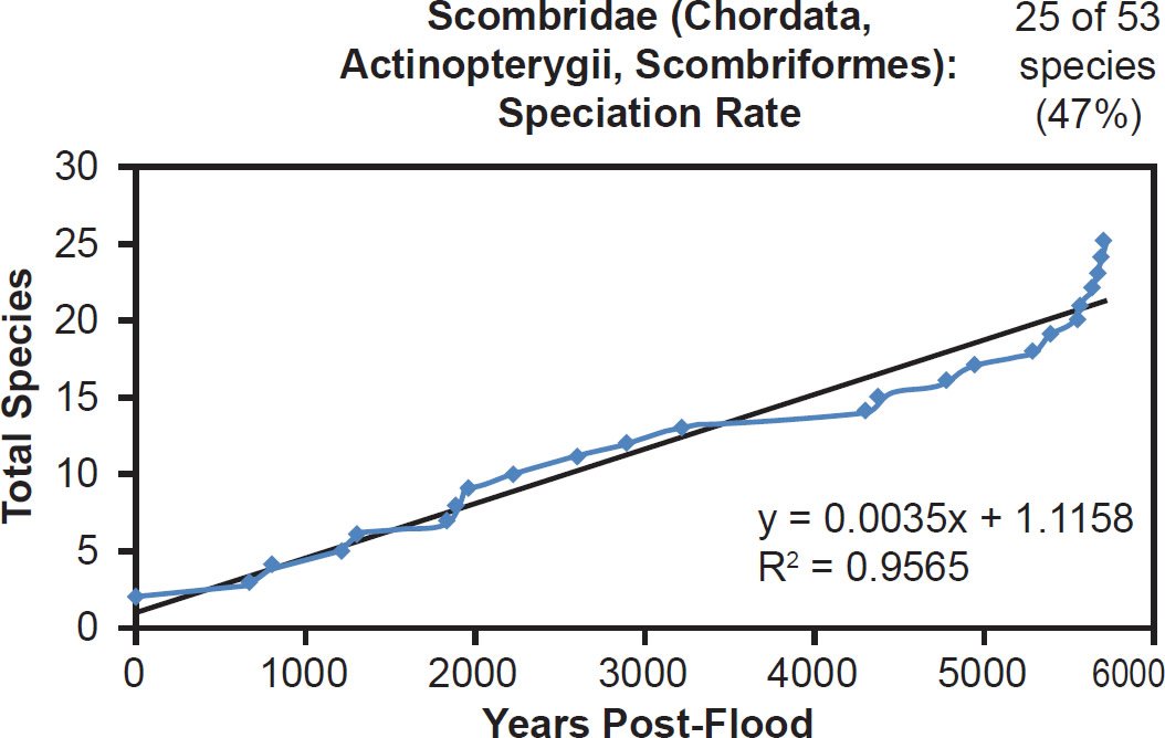
Fig. 36. Speciation rate within the family Scombridae. Whole genome alignments for extant species in the family Scombridae were performed. A phylogenetic tree was created from which branch lengths between branch points were extracted, converted to years, and used to plot the timeline of branching/speciation within the family. The results were a fairly tight fit to a linear function, which was represented by the thin black line and the equation, both of which were derived via linear regression of the raw data in Microsoft Excel. Representation of species within the family was depicted in the upper right corner.
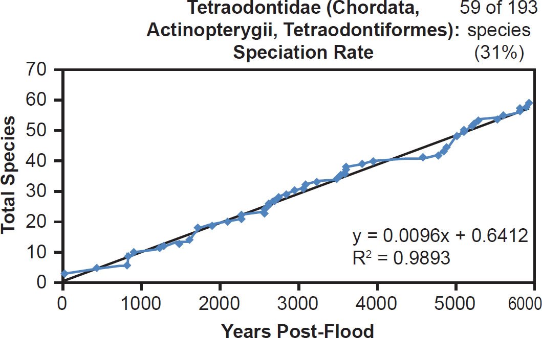
Fig. 37. Speciation rate within the family Tetraodontidae. Whole genome alignments for extant species in the family Tetraodontidae were performed. A phylogenetic tree was created from which branch lengths between branch points were extracted, converted to years, and used to plot the timeline of branching/speciation within the family. The results were a tight fit to a linear function, which was represented by the thin black line and the equation, both of which were derived via linear regression of the raw data in Microsoft Excel. Representation of species within the family was depicted in the upper right corner.
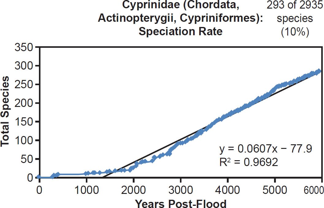
Fig. 38. Speciation rate within the family Cyprinidae. Whole genome alignments for extant species in the family Cyprinidae were performed. A phylogenetic tree was created from which branch lengths between branch points were extracted, converted to years, and used to plot the timeline of branching/speciation within the family. The results were a tight fit to a linear function, which was represented by the thin black line and the equation, both of which were derived via linear regression of the raw data in Microsoft Excel. Representation of species within the family was depicted in the upper right corner.
Linear rates were also independent of phylum. Among arthropods, linear rates described crustacean (Fig. 39) and insect speciation alike (Figs. 40–41). Among cnidarians, only a single family was analyzed, and it deviated from linear speciation hypothesis, showing evidence in favor of the late speciation hypothesis instead (Fig. 42). However, since two-thirds of the species in this analysis came from only one of the 14 Acroporidae genera, the match between the data and the late speciation hypothesis may have been an artifact of species representation. Hence, linear speciation rates described the timing of speciation within families almost entirely independent of the biology of each family.
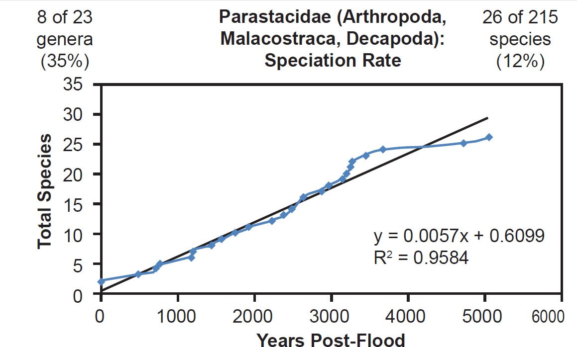
Fig. 39. Speciation rate within the family Parastacidae. Whole genome alignments for extant species in the family Parastacidae were performed. A phylogenetic tree was created from which branch lengths between branch points were extracted, converted to years, and used to plot the timeline of branching/speciation within the family. The results were a fairly tight fit to a linear function, which was represented by the thin black line and the equation, both of which were derived via linear regression of the raw data in Microsoft Excel. Representation of genera and species within the family were depicted in the upper left and right corners, respectively.
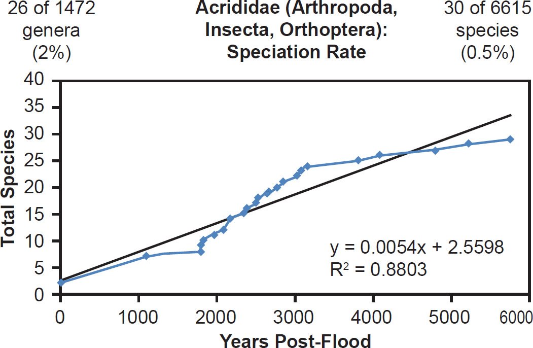
Fig. 40. Speciation rate within the family Acrididae. Whole genome alignments for extant species in the family Acrididae were performed. A phylogenetic tree was created from which branch lengths between branch points were extracted, converted to years, and used to plot the timeline of branching/speciation within the family. The results were a good fit to a linear function, which was represented by the thin black line and the equation, both of which were derived via linear regression of the raw data in Microsoft Excel. Representation of genera and species within the family were depicted in the upper left and right corners, respectively.
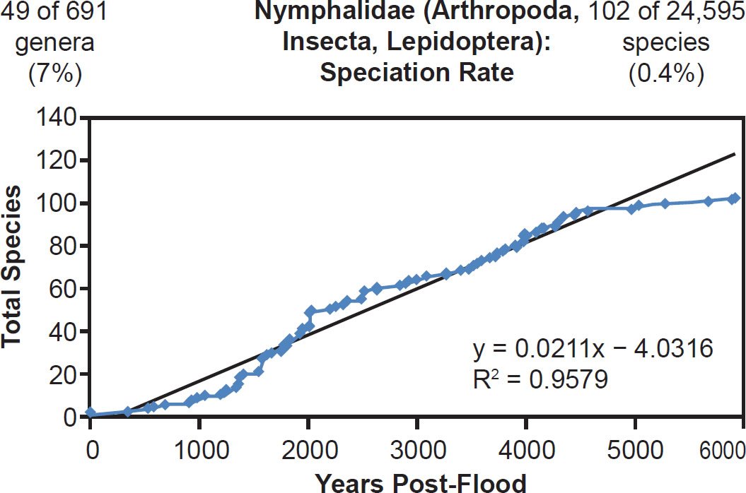
Fig. 41. Speciation rate within the family Nymphalidae. Whole genome alignments for extant species in the family Nymphalidae were performed. A phylogenetic tree was created from which branch lengths between branch points were extracted, converted to years, and used to plot the timeline of branching/speciation within the family. The results were a fairly tight fit to a linear function, which was represented by the thin black line and the equation, both of which were derived via linear regression of the raw data in Microsoft Excel. Representation of genera and species within the family were depicted in the upper left and right corners, respectively.
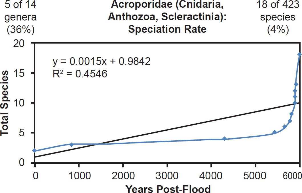
Fig. 42. Speciation rate within the family Acroporidae. Whole genome alignments for extant species in the family Acroporidae were performed. A phylogenetic tree was created from which branch lengths between branch points were extracted, converted to years, and used to plot the timeline of branching/speciation within the family. The results were a poor fit to a linear function (represented by the thin black line and the equation, both of which were derived via linear regression of the raw data in Microsoft Excel) and seemed a better fit the “Late” hypothesis (Fig. 18). Representation of genera and species within the family were depicted in the upper left and right corners, respectively.
Even the families that were mentioned in Scripture and which were previously used to argue (Wood 2002) for the early episode hypothesis showed speciation patterns that did not contradict the linear speciation rate hypothesis. As described above, the family Equidae showed a linear speciation rate (Fig. 23), and the wild horse (Equus przewalskii) branched off first from the Equid family tree (Supplemental Fig. 29). The family Camelidae had only three species total, preventing a strict graph on the timing of speciation from being drawn, yet the wild camel (Camelus ferus) branched immediately from the putative root and did not show a nested hierarchical pattern with the remaining species or any other such pattern suggestive of a later speciation event (Supplemental Fig. 49).
In families Felidae and Canidae, species representation was low, but the data still correlated well with the linear speciation rate hypothesis (Figs. 43–44).Though the wolf and lion appeared to become separate species within their respective families midway through or late in the post-Flood period, their lineages branched off early. Furthermore, it’s unclear whether the modern wolf and lion species are the same species to which Scripture refers in the passages used to argue for an early speciation event (Wood 2002). Also, in general for every speciation event, a new species splits off from a parent species, and the identity of the parental species in the wolf and lion lineages is unknown. It may have been the wolf or lion, respectively, all along. Thus, the findings of this study were not in conflict with the biblical account of the natural history of these families.
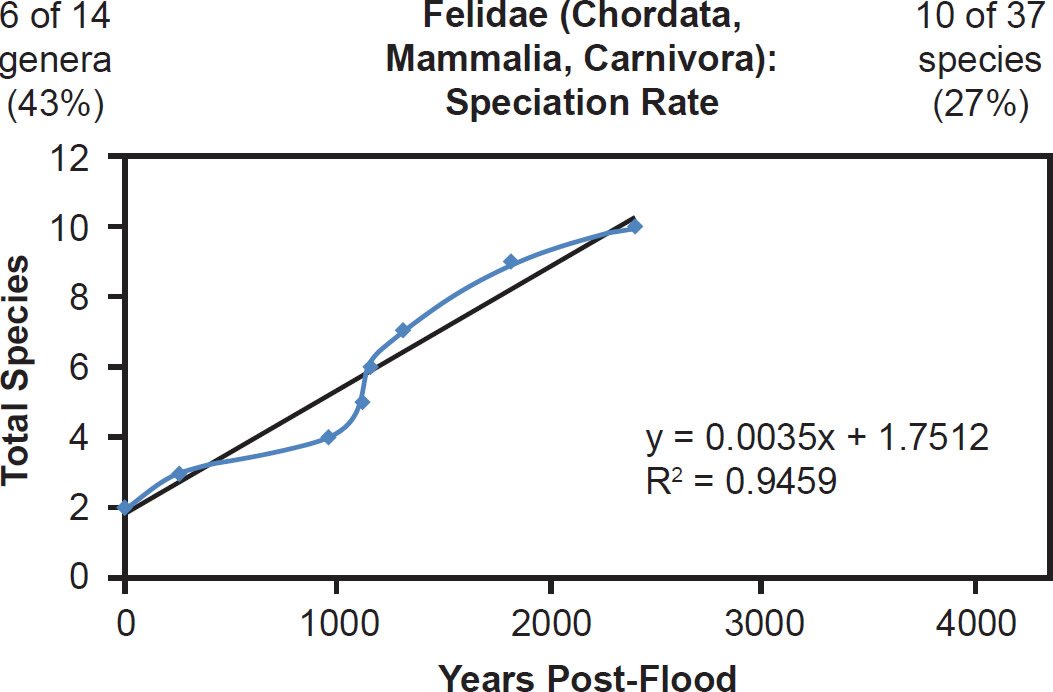
Fig. 43. Speciation rate within the family Felidae. Whole genome alignments for extant species in the family Felidae were performed. A phylogenetic tree was created from which branch lengths between branch points were extracted, converted to years, and used to plot the timeline of branching/speciation within the family. The results were a fairly tight fit to a linear function, which was represented by the thin black line and the equation, both of which were derived via linear regression of the raw data in Microsoft Excel. Representation of genera and species within the family were depicted in the upper left and right corners, respectively.
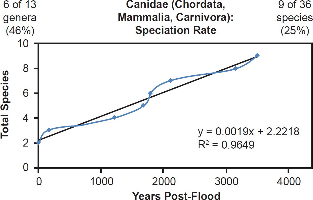
Fig. 44. Speciation rate within the family Canidae. Whole genome alignments for extant species in the family Canidae were performed. A phylogenetic tree was created from which branch lengths between branch points were extracted, converted to years, and used to plot the timeline of branching/speciation within the family. The results were a tight fit to a linear function, which was represented by the thin black line and the equation, both of which were derived via linear regression of the raw data in Microsoft Excel. Representation of genera and species within the family were depicted in the upper left and right corners, respectively.
Since linear speciation rates were found across such a diversity of taxa, the major findings of this study were generalizable into a single, testable equation: The absolute rate of speciation for extant species within a family is the division of the number of extant species within a family by the Ark-appropriate value. That is, for on-Ark families, the per-year rate of speciation is the number of extant species within the family divided by ~4350 years. For off-Ark families, the per-year rate of speciation is the number of extant species within the family divided by ~6000 years (Fig. 45A–B).
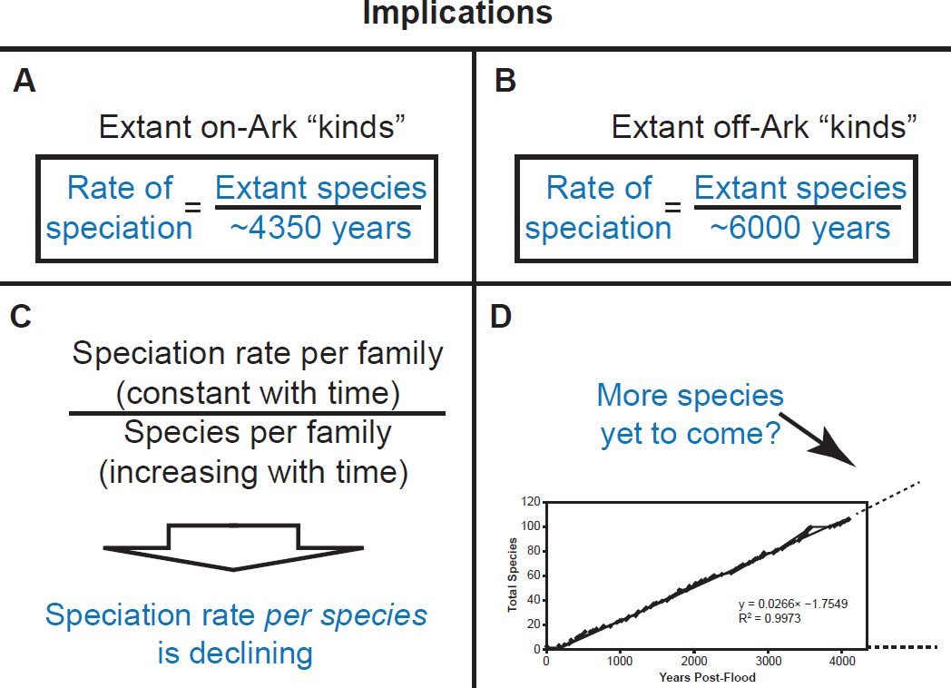
Fig. 45. Implications of the discovery of linear speciation rates within diverse families. A. If speciation rates are linear for all “kinds” taken on board the Ark, then the rate of speciation can be predicted by dividing the number of extant species by the date of the Flood (~4350 years ago). B. If speciation rates are linear for all “kinds” not taken on board the Ark, then the rate of speciation can be predicted by dividing the number of extant species by the date of Creation (~6000 years ago). C. If speciation rates are linear for all “kinds,” this means that the speciation rate per family is constant with time. However, since speciation is happening, the total number of species within the family is increasing with time. A constant numerator divided by an increasing denominator results in a quotient that is decreasing with time. Hence, if speciation rates are linear for all “kinds,” then the speciation rate per species is declining. D. If speciation rates are linear for all “kinds,” then the graphs imply that more speciation is yet to come— that speciation is still on-going and has not ceased permanently.
This was well illustrated in the mammalian families for whom all of their species were represented in the mitochondrial DNA databases. For example, in Balaenopteridae, the predicted rate of speciation (9/6000 = 0.0015) exactly matched the slope derived from linear regression of the mitochondrial DNA data (Fig. 22). Also, in the family Ursidae, the predicted rate of speciation (8/4350 = 0.0018) closely matched the slope derived from linear regression of the mitochondrial DNA data (0.0016; see Fig. 20). Finally, in the family Rhinocerotidae, the predicted rate of speciation (5/4350 = 0.0011) closely matched the slope derived from linear regression of the mitochondrial DNA data (0.0012; see Fig. 21).
To clarify, this equation makes predictions about the timing of speciation only for extant species. The total number of species within a family at any point in time includes both the still-extant species that had formed then, plus now-extinct species which were alive at the time. The equations in Fig. 45A–B make no predictions for the total number of species within a family at any point in time because the equations do not include data on now-extinct species.
A second implication of these results was that the per species speciation rates were (and are) declining. Since the speciation rates per family were constant with time but the number of species within each family was increasing with time, this effectively meant that speciation rate of each species was becoming smaller with the passage of time (Fig. 45C).
A third implication of these results was that high rates of speciation continue to this day (Fig. 45D). In contrast, the evolutionary model postulates that individual species arise over hundreds of thousands to millions of years (Futuyma 2009), implying that speciation is a rarely seen event. The equations in Fig. 45A–B estimate ongoing speciation at much faster rates. For example, within Bovidae, the predicted rate of speciation is 0.03 species per year (141/4350 = 0.03) or one new species every 31 years.
Currently, the African buffalo (Syncerus caffer) contains several subspecies, including the morphologically distinct African forest buffalo (Syncerus caffer nanus). If these subspecies become geographically (and, therefore, reproductively) isolated, they might eventually be classified as separate species, consistent with the conclusion that speciation is ongoing and observable.
As another example, the family Hominidae has a predicted rate of speciation of 0.001 (6/4350 = 0.001), or one new species every 725 years. Within the common chimpanzee species (Pan troglodytes), several subspecies exist, a fact which is immediately visible in genetics (Fig. 46, derived from the same data as Fig. 15 but rooted on the midpoint and without selecting the topology-only option in MEGA4). If the current geographic restriction (Humle et al. 2008; Oates et al. 2008; Tutin et al. 2008; Wilson et al. 2008) of these Pan troglodytes subpopulations continues, and if interbreeding among these subspecies fails to occur, new Pan species may soon emerge.
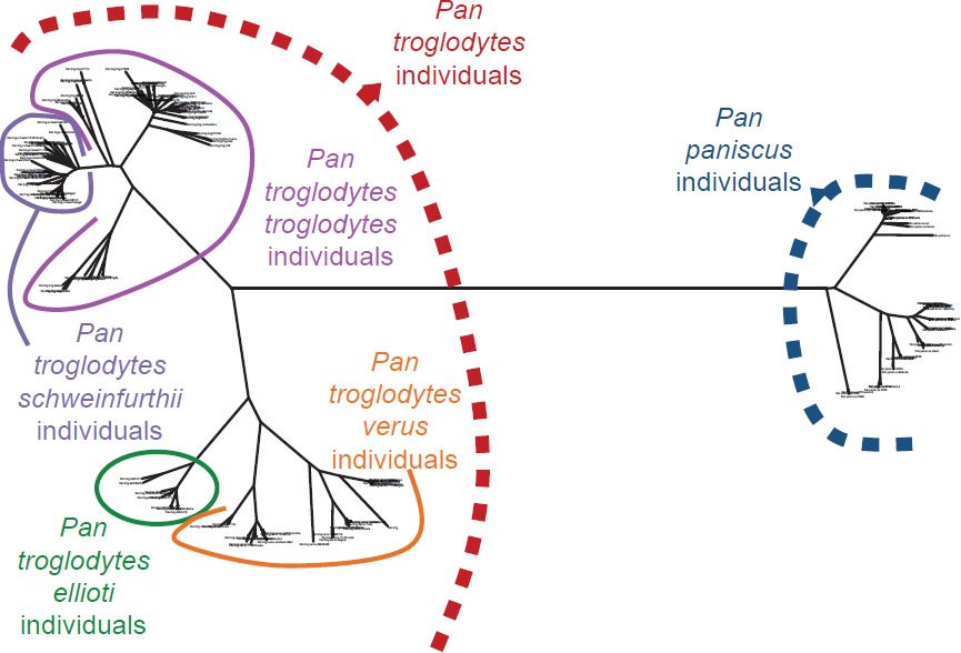
Fig. 46. Possible evidence for ongoing speciation within Pan. The same raw alignment data from which the trees in Fig. 15 were derived was used to create a mid-point rooted phylogenetic tree of members of the genus Pan. As was depicted in Fig. 15, the individuals within Pan paniscus species clearly segregated as a group from the individuals within the Pan troglodytes species. Within the latter, several subgroups were visible, corresponding to Pan troglodytes subspecies, and these subgroups may be the precursors to new Pan species.
Discussion
Ramifications for the timing of speciation
The results of this study highlight the unique advantages of genetics over the fossil record on the question of the timing of speciation. Since only a few select time points are represented in the fossil record, the history that can be inferred from paleontology is rather imprecise temporally. (This is true regardless of where the Flood/post-Flood boundary is placed in the fossil record.) Conversely, in speciose “kinds,” genetics theoretically offers many more time points. In addition, some categories of “kinds” (e.g., insects) fossilize poorly, limiting the broad taxonomic utility of paleontology. In contrast, DNA sequence information can be obtained freely in theory from nearly any species alive today. Hence, the findings of this study represent the first high resolution window in the relative timing of speciation for extant species.
Observing the past through this window revealed abundant evidence consistent with the linear speciation rate hypothesis. Nearly every family that was studied matched the expectations of the constant rate model. Although the entire dataset represented less than 30 metazoan families, the linear speciation rate results were true regardless of the classes and phyla to which these families belonged, suggesting that constant speciation rates would generally be found across most taxa. Furthermore, the results were so consistent that they led to a predictive model for the timing of speciation (Fig. 45A–B), one that can be tested with addition families in the future.
These results can be reconciled with the previous data used to argue for an early episode of speciation. As described in the Results section, the four families alluded to in Scripture (Wood 2002) did not contradict the linear speciation rate hypothesis. Also, even if the Flood/post-Flood boundary is at the K-T, the high number of species formed then may not have been the ancestors of modern extant species, which would alleviate any apparent contradiction between the paleontological findings and the present genetic findings. Finally, fossil DNA (Wood 2012, 2013b) appears to be degraded, or it may represent a group of individuals with unique and unusually high mutation rates (Fig. 11C). Neither of these scenarios undermine the foundational assumption of this study—that rates of mitochondrial DNA change in extant species have been constant through time.
Nevertheless, this assumption of constant mitochondrial DNA mutation rates could be falsified in the future by one of at least two different methods. If ancient DNA could be demonstrated to be reliable, and if it could be demonstrated that these fossil DNA sequences found immediately post-Flood were too genetically diverse to be explained by a constant rate of mutation, then the major undergirding assumption of the present study would be in error.
Alternatively, since the prospect of finding non-degraded DNA from fossils seems unlikely at present, the assumption of a constant rate of mutation could be tested with living species. By measuring the mutation rates in additional species within a family; making genetic diversity predictions from these rates under the assumption that rates have been constant; and then comparing the predictions to actual diversity, the utility of the constant rate assumption could be evaluated. If the predictions from these additional rates underestimate actual diversity within the family, then the assumption of constant rates would be falsified, and it would appear that mutation rates were higher in the past, as per Wood’s conclusions (2012, 2013b). This result would also imply that early episode (Fig. 18) speciation hypothesis was correct. Instead, if the predictions overestimated actual diversity in the family, then it would appear that either mutation rates were slower in the past or that species within a family coalesced sooner than 4350 years ago (on-Ark families)/6000 years ago (off-Ark families). This result would imply that a version of the late hypothesis (Fig. 18) was correct.
Under the assumption that molecular clocks do indeed exist, the results of this study found no evidence in support of the early episode hypothesis (Fig. 18) of Wise (1994) and Wood (2002, 2003). The fact that most vertebrate families are not highly speciose (Figs. 1–6) and that fact that nearly every family showed a linear rate of species accumulation regardless of within-family species richness (Figs. 19–44) together argued against the hypothesis that modern species arose immediately post-Flood in a burst of speciation.
Hence, it appears that speciation is not “rapid” in the sense of the early episode hypothesis (Fig. 18), but speciation does seem to happen much faster than the evolutionary community has maintained.
All of these results are dependent upon the assumption that the taxonomic rank of family is equivalent to the biblical designation of “kind,” as per previous data (Wood 2006). If “kinds” turn out to be higher or lower than the rank of family, then these results would be called into question. For highly speciose families, the possibility is especially real that the “kind” boundary may not be equivalent to the rank of family.
Nevertheless, the preliminary results in this study suggest that the conclusion of linear rates of speciation would remain intact. For example, in several of the speciose families, mitochondrial DNA representation was poor. Hence, these groups could be viewed as an approximation of a “kind” boundary lower than the rank of family. Even in these groups, linear speciation rates were still seen (e.g., Figs. 30, 38, 40–41), suggesting that linear rates of speciation were the rule even if the “kind” boundary were shifted slightly from the family rank.
Remaining questions on the timing of speciation
Several aspects of the timing of speciation were inaccessible by the methods employed in this study. First, because I assumed that the start of the speciation process was approximated by the midpoint root of each tree, it is difficult to make firm conclusions about the absolute timing of speciation. It is entirely possible that species within on-Ark “kinds” coalesce sooner than 4350 years ago and that species within off-Ark “kinds” coalesce sooner than 6000 years ago.
If these hypotheses are true, a linear pattern would still be present within these families, but only for the length of time that speciation was happening. In a sense, this result would be a fusion of the linear and late hypotheses. Under this scenario, speciation events would begin late post-Flood, but, once they began, they would follow a linear pattern. Hence, anchoring the linear patterns discovered in this study to absolute dates on the YE timescale will require further study.
Evaluation might begin by comparing the predictions from the equations in Fig. 45A–B to recorded history. In addition, mitochondrial DNA mutation rates could be measured for several species within each family to see if the predictions from these rates overestimate or accurately describe the genetic diversity within the family. If the predictions matched the actual diversity, this would support the assumptions made in this study and the timestamps assigned to the various speciation events.
Despite these concerns, the preliminary results of this study suggest that, for several “kinds,” the timelines I depicted (Figs. 19–44) were not too far off the absolute timescale. For example, among the on-Ark carnivores (Fig. 13), the various families were separated from one another by few DNA differences. In contrast, species within families were sometimes separated by large DNA differences. Had speciation commenced late post-Flood, then I would have expected the DNA differences between species to have been less than the DNA differences between families.
Second, the timing of speciation for extinct families is also inaccessible by this study. Since I limited my analyses to extant species, these results say nothing about the timing of speciation for “kinds” which did not survive to today.
Third, these results are silent on the question of the rates of speciation for now-extinct species in still-extant families. Presumably, if DNA data were available for these extinct species, the fact of linear rates would remain, and only the slopes/absolute values for the rates of speciation would need to be modified. In a sense, the speciose-families with poor DNA sequence representation (Figs. 30, 38, 40–41) are already a model of this scenario. I anticipate that the addition of more DNA sequences from extant species to these family calculations will simply change the slope and not the linear structure of the graph.
Finally, these studies do not directly address why some families became very speciose and others remained/are species-poor. The power distribution seems to approximate the species per family in a variety of taxonomic groups, but the reason why this function fits the data best remains unknown.
Ramifications for the mechanism of speciation
The results of this study put several of the prevailing hypotheses on the mechanism of speciation in a new light. The equations in Fig. 45A–B indicate that the rate of speciation is predictable from the total number of species within a family. Since species within a family occupy diverse environments, it would appear that the rate of speciation within a family is not predictable from the type of environments that the family may have encountered during its history. This suggests that speciation may not be a process of directed mutation in response to environmental challenges.
Furthermore, since the rate of speciation appears to be constant, rather than an exponential function which eventually trails off with time, the need for creative mechanisms of speciation appears to be obviated. Since some of the most inventive mechanistic hypotheses were created to explain the early episode hypothesis of speciation (Fig. 18), the fact of linear speciation rates implies that novel proposals are no longer required. Specifically, this would suggest that transposon-mediated mechanisms (e.g., Terborg 2008, 2009; Shan 2009; Wood 2002, 2003) are not needed for speciation.
Nevertheless, the fact of chromosomal differences among species may still necessitate unique proposals on genetic change (Wood 2013a).
By contrast, the linear speciation rate results in the present study implicate a mechanism that has existed in the creationist community for decades (e.g., Parker 1980)—a hypothesis termed “heterozygous fractionation” (Wood 2002). Under this hypothesis, God created the first individuals within each “kind” with heterozygosity in their nuclear DNA compartment. This genetic diversity represents the raw material to be reshuffled each generation, and the process of recombination ultimately leads to morphologically distinct individuals that form populations which we would label separate “species.”
Though the focus in this study was mitochondrial DNA, the principles about the timing of speciation that were inferred from these data were consistent with several expectations of the heterozygous fractionation hypothesis for nuclear DNA. First, under this hypothesis, fractionating the originally diverse pool of nuclear alleles would likely dilute the potential for speciation within each new species. Since each new species would contain a fraction of the original nuclear allele pool, the number of available nuclear alleles for recombination would become smaller with each new speciation event. This would effectively lower the speciation potential with each new speciation event, consistent with the results of this study that indicate that the rate of speciation per species is declining (Fig. 45C).
Second, on the flip side, under the heterozygous fractionation hypothesis, speciation would be ongoing. Since it’s not driven by any unique environmental trigger or by one-time historical events, new species could form, theoretically, at any time so long as sufficient alleles are present for recombination to produce new varieties. The results of this study suggest that speciation is ongoing (Fig. 45D).
Third, independent of the results of this study, precise accounting for the current set of alleles in the human population nearly requires an initially heterozygous pair (Carter 2011). If humans were created heterozygous, perhaps the animals “kinds” were as well.
Fractionation of a heterozygous allele pool is also a feasible explanation. Population genetics has identified the conditions required to prevent fractionation of heterozygosity—conditions termed “the Hardy-Weinberg principle” (Futuyma 2009). If a population of individuals is infinite in size, if mating among individuals occurs randomly and without inbreeding, if the species is not broken up into different isolated subpopulations (migration and gene flow reduce boundaries between subpopulations), if mutation does not occur, and if natural selection does not happen, then heterozygosity will be maintained, and no change in the frequency of alleles in the population will occur. Obviously, these conditions do not exist anywhere on earth, which means that all initially heterozygous populations will change over time as they reproduce. In other words, if God created the first members of each “kind” as heterozygous individuals, then He virtually ensured that genetic drift—and, as a likely result, speciation—would occur.
Ironically, heterozygous fractionation via genetic drift is an explanation that, in one sense, fits the parameters that Wise (1994) outlined previously. Drift and fractionation are ultimately intrinsic mechanisms of speciation, but they follow from the linear speciation rate hypothesis rather than the rapid speciation hypothesis that Wise articulated.
Since the linear speciation rate hypothesis fit such a diversity of families, this result suggests that the mechanism driving speciation is consistent across a diversity of families. Hence, at the present, genetic drift of created heterozygosity seems to be the best explanation for the process of speciation worldwide. Why certain “kinds” have drifted more than others remains unanswered, and further research is needed to see just how generalizable this explanation is and to explore additional lines of evidence that may confirm or falsify the heterozygous fractionation and genetic drift hypothesis.
Conclusion
Mitochondrial DNA patterns within families indicate that the speciation process which has led to the origin of extant species has occurred at constant rates. This finding was true in families belonging to diverse taxa, suggesting that it was independent of the means by which “kinds” survived the Flood, independent of their intra-“kind” species richness, and independent of their taxon-specific biology. Furthermore, it suggested that the mechanism of speciation was shared across diverse “kinds” and that this mechanism might be genetic drift of created heterozygosity.
Acknowledgments
Jason Lisle was instrumental in deriving the conclusion that speciation rates per species are declining, and he was a key consultant on many other facets of this undertaking. Rob Carter always provided unique and invaluable feedback on the many genetic aspects of this study, particularly on the details of population genetics. A preliminary version of this work was presented at the 2014 Creation Research Society meeting, and feedback from the attendees there was helpful in refining the conclusions. Special thanks to the reviewers who also helped refine the conclusions in this paper.
References
Austin, S. A., J. R. Baumgardner, D. R. Humphreys, A. A. Snelling, L. Vardiman, and K. P. Wise. 1994. “Catastrophic Plate Tectonics: A Global Flood Model of Earth History.” In Proceedings of the Third International Conference on Creationism. Edited by R. E. Walsh, 609–21. Pittsburgh, Pennsylvania: Creation Science Fellowship.
Carter, R. W. 2007. “Mitochondrial Diversity Within Modern Human Populations.” Nucleic Acids Research 35 (9): 3039– 045.
Carter, R. W. 2010. “Adam, Eve and Noah vs Modern Genetics.” Accessed February 25, 2015. http://creation.com/noah-and-genetics.
Carter, R. W. 2011. “The Non-Mythical Adam and Eve! Refuting errors by Francis Collins and BioLogos.” Accessed March 4, 2015. http://creation.com/historical-adam-biologos.
Carter, R. W., D. Criswell, and J. Sanford. 2008. “The ‘Eve’ Mitochondrial Consensus Sequence.” In Proceedings of the Sixth International Conference on Creationism. Edited by A. A. Snelling, 111–16. Pittsburgh, Pennsylvania: Creation Science Fellowship and Dallas, Texas: Institute for Creation Research.
Cavanaugh, D. P., T. C. Wood, and K. P. Wise. 2003. “Fossil Equidae: A Monobaraminic, Stratomorphic Series.” In Proceedings of the Fifth International Conference on Creationism. Edited by R. L. Ivey Jr., 143–54. Pittsburgh, Pennsylvania: Creation Science Fellowship.
Criswell, D. 2009. “Neandertal DNA and Modern Humans.” Creation Research Society Quarterly 45 (4): 246–54.
Darwin, C. 1859. On the Origin of Species by Means of Natural Selection, Or, The Preservation of Favoured Races in the Struggle for Life. London, England: John Murray.
Dawkins, R. 2009. The Greatest Show on Earth: The Evidence for Evolution. New York, New York: Free Press.
Futuyma, D. J. 2009. Evolution. Sunderland, Massachusetts: Sinauer Associates, Inc.
Gates, C., and K. Aune. 2008. Bison bison. The IUCN Red List of Threatened Species. Version 2014.3. Accessed February 26, 2015. www.iucnredlist.org.
Gates, C. C., C. H. Freese, P. J. P. Gogan, and M. Kotzman, (eds. and comps.) 2010. American Bison: Status Survey and Conservation Guidelines 2010. Gland, Switzerland: IUCN. Accessed February 25, 2015. http://www.iucn.org/knowledge/publications_doc/publications/?4878/American-bison--status-survey-and-conservation-guidelines-2010.
Hardy, C., and R. Carter. 2014. “The Biblical Minimum and Maximum Age of the Earth.” Journal of Creation 28 (2): 89–96.
Hinch, A. G., A. Tandon, N. Patterson, Y. Song, N. Rohland, C. D. Palmer, G. K. Chen, et al. 2011. “The Landscape of Recombination in African Americans.” Nature 476 (7359): 170–75.
Ho, S. Y. W. 2014. “The Changing Face of the Molecular Evolutionary Clock.” Trends in Ecology & Evolution 29 (9): 496–503.
Holt, R. D. 1996. “Evidence for a Late Cainozoic Flood/Post- Flood Boundary.” Creation Ex Nihilo Technical Journal 10 (1): 128–67.
Humle, T., C. Boesch, C. Duvall, C. M. Ellis, K. H. Farmer, I. Herbinger, A. Blom, and J. F. Oates. 2008. Pan troglodytes ssp. verus. The IUCN Red List of Threatened Species. Version 2014.3. Accessed March 2, 2015. www.iucnredlist.org.
Ingman, M., H. Kaessmann, S. Pääbo, and U. Gyllensten. 2000. “Mitochondrial Genome Variation and the Origin of Modern Humans.” Nature 408 (6813): 708–13.
IUCN SSC Antelope Specialist Group. 2008. Syncerus caffer. The IUCN Red List of Threatened Species. Version 2014.3. Accessed February 26, 2015. www.iucnredlist.org.
Jeanson, N. T. 2013. “Recent, Functionally Diverse Origin for Mitochondrial Genes from ~2700 Metazoan Species.” Answers Research Journal 6: 467–501. https://answersingenesis.org/genetics/mitochondrial-dna/recent-functionally-diverse-origin-for-mitochondrial-genes-from-~2700-metazoan-species/.
Lightner, J. K. 2009. “Gene Duplications and Nonrandom Mutations in the Family Cercopithecidae: Evidence for Designed Mechanisms Driving Adaptive Genomic Mutations.” Creation Research Society Quarterly 46 (1): 1–5.
Mack, R. 1970. “The Great African Cattle Plague Epidemic of the 1890’s.” Tropical Animal and Health Production 2 (4): 210–19.
McGee, D. 2012. “Creation Date of Adam From the Perspective of Young-Earth Creationism.” Answers Research Journal 5: 217–30. https://answersingenesis.org/bible-characters/adam-and-eve/creation-date-of-adam-from-young-earth-creationism-perspective/.
Oard, M. J. 2007. “Defining the Flood/Post-Flood Boundary in Sedimentary Rocks.” Journal of Creation 21 (1): 98–110.
Oates, J. F., A. Dunn, E. Greengrass, and B. J. Morgan. 2008. Pan troglodytes ssp. ellioti. The IUCN Red List of Threatened Species. Version 2014.3. Accessed March 2, 2015. www.iucnredlist.org.
Parker, G. 1980. “Creation, Mutation, and Variation.” Acts & Facts 9:11.
Ross, M. 2014. “Reliable Data Disconfirm a Late Cenozoic Post-Flood Boundary.” Journal of Creation 28 (2): 66–68.
Shan, E. L. 2009. “Transposon Amplification in Rapid Intrabaraminic Diversification.” Journal of Creation 23 (2): 110–17.
Terborg, P. 2008. “Evidence for the Design of Life: Part 2—Baranomes.” Journal of Creation 22 (3): 68–76.
Terborg, P. 2009. “The Design of Life: Part 3—An Introduction to Variation-Inducing Genetic Elements.” Journal of Creation 23 (1): 99–106.
Thomas, B., and J. Tomkins. 2014. “How Reliable are Genomes from Ancient DNA?” Journal of Creation 28 (3): 92–98.
Tutin, C. E. G., J. E. M. Baillie, J. Dupain, S. Gatti, F. Maisels, E. J. Stokes, D. B. Morgan, and P. D. Walsh. 2008. Pan troglodytes ssp. troglodytes. The IUCN Red List of Threatened Species. Version 2014.3. Accessed March 2, 2015. www.iucnredlist.org.
Whitmore, J. H., and P. Garner. 2008. “Using Suites of Criteria to Recognize Pre-Flood, Flood, and Post-Flood Strata in the Rock Record with Application to Wyoming (USA).” In Proceedings of the Sixth International Conference on Creationism. Edited by A. A. Snelling, 425–48. Pittsburgh, Pennsylvania: Creation Science Fellowship and Dallas, Texas: Institute for Creation Research.
Whitmore, J. H., and K. P. Wise. 2008. “Rapid and Early Post- Flood Mammalian Diversification Evidenced in the Green River Formation.” In Proceedings of the Sixth International Conference on Creationism. Edited by A. A. Snelling, 449–57. Pittsburgh, Pennsylvania: Creation Science Fellowship and Dallas, Texas: Institute for Creation Research.
Wilson, M. L., Z. Balmforth, D. Cox, T. Davenport, J. Hart, C. Hicks, K. D. Hunt, et al. 2008. Pan troglodytes ssp. schweinfurthii. The IUCN Red List of Threatened Species. Version 2014.3. Accessed March 2, 2015. www.iucnredlist.org.
Wise, K. P. 1994. “Australopithecus ramidus and the Fossil Record.” Creation Ex Nihilo Technical Journal 8 (2): 160–65.
Wise, K. P. 2005. “The Flores Skeleton and Human Baraminology.” Occasional Papers of the BSG 6: 1–13.
Wood T. C. 2002. “The AGEing Process: Rapid Post-Flood, Intrabaraminic Diversification Caused by Altruistic Genetic Elements (AGEs).” Origins (GRI) 54: 5–34.
Wood, T. C. 2003. “Perspectives on AGEing, a Young-Earth Creation Diversification Model.” In Proceedings of the Fifth International Conference on Creationism. Edited by R. L. Ivey Jr., 479–89. Pittsburgh, Pennsylvania: Creation Science Fellowship.
Wood, T. C. 2006. “The Current Status of Baraminology.” Creation Research Society Quarterly 43 (3): 149–58.
Wood, T. C. 2011. “Terrestrial Mammal Families and Creationist Perspectives on Speciation.” Journal of Creation Theology and Science Series B: Life Sciences 1: 2–5.
Wood, T. C. 2012. “Ancient mtDNA Implies a Nonconstant Molecular Clock in the Human Holobaramin.” Journal of Creation Theology and Science Series B: Life Sciences 2: 18–26.
Wood, T. C. 2013a. “A Review of the Last Decade of Creation Biology Research on Natural History, 2003–2012.” In Proceedings of the Seventh International Conference on Creationism. Edited by M. Horstemeyer. Pittsburgh, Pennsylvania: Creation Science Fellowship.
Wood, T. C. 2013b. “Mitochondrial DNA Analysis of Three Terrestrial Mammal Baramins (Equidae, Felidae, and Canidae) Implies an Accelerated Mutation Rate Near the Time of the Flood.” In Proceedings of the Seventh International Conference on Creationism. Edited by M. Horstemeyer. Pittsburgh, Pennsylvania: Creation Science Fellowship.
Supplemental Files
Supplemental Fig. 1. Radiation style tree of species within the family Bovidae. Mitochondrial DNA whole genome alignments were performed, and the resultant alignment file was used to create a radiation style tree.
Supplemental Fig. 2. Radiation style tree of species within the family Ursidae. Mitochondrial DNA whole genome alignments were performed, and the resultant alignment file was used to create a radiation style tree.
Supplemental Fig. 3. Radiation style tree of species within the family Rhinocerotidae. Mitochondrial DNA whole genome alignments were performed, and the resultant alignment file was used to create a radiation style tree.
Supplemental Fig. 4. Radiation style tree of species within the family Balaenopteridae. Mitochondrial DNA whole genome alignments were performed, and the resultant alignment file was used to create a radiation style tree.
Supplemental Fig. 5. Radiation style tree of species within the family Equidae. Mitochondrial DNA whole genome alignments were performed, and the resultant alignment file was used to create a radiation style tree.
Supplemental Fig. 6. Radiation style tree of species within the family Hominidae. Mitochondrial DNA whole genome alignments were performed, and the resultant alignment file was used to create a radiation style tree.
Supplemental Fig. 7. Radiation style tree of species within the family Phocidae. Mitochondrial DNA whole genome alignments were performed, and the resultant alignment file was used to create a radiation style tree.
Supplemental Fig. 8. Radiation style tree of species within the family Cervidae. Mitochondrial DNA whole genome alignments were performed, and the resultant alignment file was used to create a radiation style tree.
Supplemental Fig. 9. Radiation style tree of species within the family Cercopithecidae. Mitochondrial DNA whole genome alignments were performed, and the resultant alignment file was used to create a radiation style tree.
Supplemental Fig. 10. Radiation style tree of species within the family Mustelidae. Mitochondrial DNA whole genome alignments were performed, and the resultant alignment file was used to create a radiation style tree.
Supplemental Fig. 11. Radiation style tree of species within the family Delphinidae. Mitochondrial DNA whole genome alignments were performed, and the resultant alignment file was used to create a radiation style tree.
Supplemental Fig. 12. Radiation style tree of species within the family Muridae. Mitochondrial DNA whole genome alignments were performed, and the resultant alignment file was used to create a radiation style tree.
Supplemental Fig. 13. Radiation style tree of species within the family Gruidae. Mitochondrial DNA whole genome alignments were performed, and the resultant alignment file was used to create a radiation style tree.
Supplemental Fig. 14. Radiation style tree of species within the family Phasianidae. Mitochondrial DNA whole genome alignments were performed, and the resultant alignment file was used to create a radiation style tree. Rather than genus-species names, the NCBI accession information was displayed for each species.
Supplemental Fig. 15. Radiation style tree of species within the family Crocodylidae. Mitochondrial DNA whole genome alignments were performed, and the resultant alignment file was used to create a radiation style tree.
Supplemental Fig. 16. Radiation style tree of species within the family Hynobiidae. Mitochondrial DNA whole genome alignments were performed, and the resultant alignment file was used to create a radiation style tree.
Supplemental Fig. 17. Radiation style tree of species within the family Anguillidae. Mitochondrial DNA whole genome alignments were performed, and the resultant alignment file was used to create a radiation style tree.
Supplemental Fig. 18. Radiation style tree of species within the family Scombridae. Mitochondrial DNA whole genome alignments were performed, and the resultant alignment file was used to create a radiation style tree. Rather than genus-species names, the NCBI accession information was displayed for each species.
Supplemental Fig. 19. Radiation style tree of species within the family Tetraodontidae. Mitochondrial DNA whole genome alignments were performed, and the resultant alignment file was used to create a radiation style tree.
Supplemental Fig. 20. Radiation style tree of species within the family Cyprinidae. Mitochondrial DNA whole genome alignments were performed, and the resultant alignment file was used to create a radiation style tree.
Supplemental Fig. 21. Radiation style tree of species within the family Parastacidae. Mitochondrial DNA whole genome alignments were performed, and the resultant alignment file was used to create a radiation style tree. Rather than genus-species names, the NCBI accession information was displayed for each species.
Supplemental Fig. 22. Radiation style tree of species within the family Acrididae. Mitochondrial DNA whole genome alignments were performed, and the resultant alignment file was used to create a radiation style tree. Rather than genus-species names, the NCBI accession information was displayed for each species.
Supplemental Fig. 23. Radiation style tree of species within the family Nymphalidae. Mitochondrial DNA whole genome alignments were performed, and the resultant alignment file was used to create a radiation style tree. Rather than genus-species names, the NCBI accession information was displayed for each species.
Supplemental Fig. 24. Radiation style tree of species within the family Acroporidae. Mitochondrial DNA whole genome alignments were performed, and the resultant alignment file was used to create a radiation style tree. Rather than genus-species names, the NCBI accession information was displayed for each species.
Supplemental Fig. 25. Linearized and mid-point rooted tree of species within the family Bovidae. Mitochondrial DNA whole genome alignments were performed, and the resultant alignment file was used to create a linearized, mid-point rooted tree with branch lengths displayed. The mid-point root was assumed to represent the start of the speciation process.
Supplemental Fig. 26. Linearized and mid-point rooted tree of species within the family Ursidae. Mitochondrial DNA whole genome alignments were performed, and the resultant alignment file was used to create a linearized, mid-point rooted tree with branch lengths displayed. The mid-point root was assumed to represent the start of the speciation process.
Supplemental Fig. 27. Linearized and mid-point rooted tree of species within the family Rhinocerotidae. Mitochondrial DNA whole genome alignments were performed, and the resultant alignment file was used to create a linearized, mid-point rooted tree with branch lengths displayed. The mid-point root was assumed to represent the start of the speciation process.
Supplemental Fig. 28. Linearized and mid-point rooted tree of species within the family Balaenopteridae. Mitochondrial DNA whole genome alignments were performed, and the resultant alignment file was used to create a linearized, mid-point rooted tree with branch lengths displayed. The mid-point root was assumed to represent the start of the speciation process.
Supplemental Fig. 29. Linearized and mid-point rooted tree of species within the family Equidae. Mitochondrial DNA whole genome alignments were performed, and the resultant alignment file was used to create a linearized, mid-point rooted tree with branch lengths displayed. The mid-point root was assumed to represent the start of the speciation process.
Supplemental Fig. 30. Linearized and mid-point rooted tree of species within the family Hominidae. Mitochondrial DNA whole genome alignments were performed, and the resultant alignment file was used to create a linearized, mid-point rooted tree with branch lengths displayed. The mid-point root was assumed to represent the start of the speciation process.
Supplemental Fig. 31. Linearized and mid-point rooted tree of species within the family Phocidae. Mitochondrial DNA whole genome alignments were performed, and the resultant alignment file was used to create a linearized, mid-point rooted tree with branch lengths displayed. The mid-point root was assumed to represent the start of the speciation process.
Supplemental Fig. 32. Linearized and mid-point rooted tree of species within the family Cervidae. Mitochondrial DNA whole genome alignments were performed, and the resultant alignment file was used to create a linearized, mid-point rooted tree with branch lengths displayed. The mid-point root was assumed to represent the start of the speciation process.
Supplemental Fig. 33. Linearized and mid-point rooted tree of species within the family Cercopithecidae. Mitochondrial DNA whole genome alignments were performed, and the resultant alignment file was used to create a linearized, mid-point rooted tree with branch lengths displayed. The mid-point root was assumed to represent the start of the speciation process.
Supplemental Fig. 34. Linearized and mid-point rooted tree of species within the family Mustelidae. Mitochondrial DNA whole genome alignments were performed, and the resultant alignment file was used to create a linearized, mid-point rooted tree with branch lengths displayed. The mid-point root was assumed to represent the start of the speciation process.
Supplemental Fig. 35. Linearized and mid-point rooted tree of species within the family Delphinidae. Mitochondrial DNA whole genome alignments were performed, and the resultant alignment file was used to create a linearized, mid-point rooted tree with branch lengths displayed. The mid-point root was assumed to represent the start of the speciation process.
Supplemental Fig. 36. Linearized and mid-point rooted tree of species within the family Muridae. Mitochondrial DNA whole genome alignments were performed, and the resultant alignment file was used to create a linearized, mid-point rooted tree with branch lengths displayed. The mid-point root was assumed to represent the start of the speciation process.
Supplemental Fig. 37. Linearized and mid-point rooted tree of species within the family Gruidae. Mitochondrial DNA whole genome alignments were performed, and the resultant alignment file was used to create a linearized, mid-point rooted tree with branch lengths displayed. The mid-point root was assumed to represent the start of the speciation process.
Supplemental Fig. 38. Linearized and mid-point rooted tree of species within the family Phasianidae. Mitochondrial DNA whole genome alignments were performed, and the resultant alignment file was used to create a linearized, mid-point rooted tree with branch lengths displayed. The mid-point root was assumed to represent the start of the speciation process. Rather than genus-species names, the NCBI accession information was displayed for each species.
Supplemental Fig. 39. Linearized and mid-point rooted tree of species within the family Crocodylidae. Mitochondrial DNA whole genome alignments were performed, and the resultant alignment file was used to create a linearized, mid-point rooted tree with branch lengths displayed. The mid-point root was assumed to represent the start of the speciation process.
Supplemental Fig. 40. Linearized and mid-point rooted tree of species within the family Hynobiidae. Mitochondrial DNA whole genome alignments were performed, and the resultant alignment file was used to create a linearized, mid-point rooted tree with branch lengths displayed. The mid-point root was assumed to represent the start of the speciation process.
Supplemental Fig. 41. Linearized and mid-point rooted tree of species within the family Anguillidae. Mitochondrial DNA whole genome alignments were performed, and the resultant alignment file was used to create a linearized, mid-point rooted tree with branch lengths displayed. The mid-point root was assumed to represent the start of the speciation process.
Supplemental Fig. 42. Linearized and mid-point rooted tree of species within the family Scombridae. Mitochondrial DNA whole genome alignments were performed, and the resultant alignment file was used to create a linearized, mid-point rooted tree with branch lengths displayed. The mid-point root was assumed to represent the start of the speciation process. Rather than genus-species names, the NCBI accession information was displayed for each species.
Supplemental Fig. 43. Linearized and mid-point rooted tree of species within the family Tetraodontidae. Mitochondrial DNA whole genome alignments were performed, and the resultant alignment file was used to create a linearized, mid-point rooted tree with branch lengths displayed. The mid-point root was assumed to represent the start of the speciation process.
Supplemental Fig. 44. Linearized and mid-point rooted tree of species within the family Cyprinidae. Mitochondrial DNA whole genome alignments were performed, and the resultant alignment file was used to create a linearized, mid-point rooted tree with branch lengths displayed. The mid-point root was assumed to represent the start of the speciation process.
Supplemental Fig. 45. Linearized and mid-point rooted tree of species within the family Parastacidae. Mitochondrial DNA whole genome alignments were performed, and the resultant alignment file was used to create a linearized, mid-point rooted tree with branch lengths displayed. The mid-point root was assumed to represent the start of the speciation process. Rather than genus-species names, the NCBI accession information was displayed for each species.
Supplemental Fig. 46. Linearized and mid-point rooted tree of species within the family Acrididae. Mitochondrial DNA whole genome alignments were performed, and the resultant alignment file was used to create a linearized, mid-point rooted tree with branch lengths displayed. The mid-point root was assumed to represent the start of the speciation process. Rather than genus-species names, the NCBI accession information was displayed for each species.
Supplemental Fig. 47. Linearized and mid-point rooted tree of species within the family Nymphalidae. Mitochondrial DNA whole genome alignments were performed, and the resultant alignment file was used to create a linearized, mid-point rooted tree with branch lengths displayed. The mid-point root was assumed to represent the start of the speciation process. Rather than genus-species names, the NCBI accession information was displayed for each species.
Supplemental Fig. 48. Linearized and mid-point rooted tree of species within the family Acroporidae. Mitochondrial DNA whole genome alignments were performed, and the resultant alignment file was used to create a linearized, mid-point rooted tree with branch lengths displayed. The mid-point root was assumed to represent the start of the speciation process. Rather than genus-species names, the NCBI accession information was displayed for each species.
Supplemental Fig. 49. Radiation style tree of species within the family Camelidae. Mitochondrial DNA whole genome alignments were performed, and the resultant alignment file was used to create a radiation style tree.
Supplemental Fig. 50. Radiation style tree of species within the family Felidae. Mitochondrial DNA whole genome alignments were performed, and the resultant alignment file was used to create a radiation style tree.
Supplemental Fig. 51. Radiation style tree of species within the family Canidae. Mitochondrial DNA whole genome alignments were performed, and the resultant alignment file was used to create a radiation style tree.
Supplemental Fig. 52. Linearized and mid-point rooted tree of species within the family Felidae. Mitochondrial DNA whole genome alignments were performed, and the resultant alignment file was used to create a linearized, mid-point rooted tree with branch lengths displayed. The mid-point root was assumed to represent the start of the speciation process.
Supplemental Fig. 53. Linearized and mid-point rooted tree of species within the family Canidae. Mitochondrial DNA whole genome alignments were performed, and the resultant alignment file was used to create a linearized, mid-point rooted tree with branch lengths displayed. The mid-point root was assumed to represent the start of the speciation process.
Supplemental Table 1. Common names for taxonomic groups and species used in this study.
Supplemental Table 2. Taxonomic information from IUCN for species within Mammalia.
Supplemental Table 3. Taxonomic information from the Reptile Database for species within Reptilia.
Supplemental Table 4. Taxonomic information from the Amphibian Species of the World list for species within Amphibia.
Supplemental Table 5. Taxonomic information from the BirdLife Checklist for species within Aves.
Supplemental Table 6. Taxonomic information from the Catalog of Fishes for members of Actinopterygii.
Supplemental Table 7. NCBI accession numbers for all sequences used in this paper.
Supplemental Table 8. Raw calculations for mitochondrial DNA clock predictions.
Supplemental Table 9. D-loop sequence differences among human non-African ethnic groups.