Numerical Modeling of the Large-Scale Erosion, Sediment Transport, and Deposition Processes of the Genesis Flood

Note: This paper has been revised. After the paper’s publication the author discovered a problem in the numerical formulation that invalidated some of the paper’s main conclusions. The reader is encouraged to refer to the revised version in which the numerical problem has been repaired.

Introduction

Accounting for the thick sediment sequences that blanket the surfaces of the continents is a paramount issue for understanding the physical aspects of the Genesis Flood. In continental platform regions, such as the heartland of the U.S., the sequence of fossil-bearing sediment layers are commonly 2000 m (6561 ft) or more in cumulative thickness (Prothero and Schwab 2004, 12–14). They also typically display astonishing horizontal continuity (e.g., Ager 1973). Just what sort of physical processes could have moved such huge volumes of sediment and arranged it in such orderly, laterally extensive layers within the span of a single year, as Scripture requires? As a preliminary exercise one can make rough estimates of the erosion, sediment transport, and deposition rates that are needed. If we assume that most of the primary deposition occurred within the interval of 150 days during which “the water prevailed on the earth” (Genesis 7:24), we can compute an average deposition rate over that interval needed to produce a column of sediment, say, 1800 m (5905 ft) thick, which is the mean value over the continents today. Dividing 1800 m (5905 ft) by 150 days yields a time-averaged rate of deposition of 12 m/day (0.5 m/hr or 1.4 × 10^-4 m/s). It also suggests a comparable time-averaged rate of erosion.

The large lateral extent of most of the layers suggests significant transport distances. Let us assume that the average distance between the sites of erosion and deposition is 1000 km (621 mi) (1 × 10⁶ m) and that the average speed of the water is 20 m/s (45 mph). A typical sediment particle is therefore in suspension for (1 × 10⁶ m)/(20 m/s) = 5 × 10⁴ s (13.9 hr). If the input and output of the pipeline, so to speak, is the erosion/deposition rate of 1.4 × 10^-4 m/s, then the average suspended sediment load distributed vertically through the sheet of flowing water must be (1.4 × 10^-4 m/s) × (5 × 10⁴ s) = 7 m. This requires that the depth of the flowing water be great enough and also its turbulence intense enough to sustain this sort of suspended load. From these simple estimates it is obvious that any viable candidate mechanism likely involves coherent sheets of turbulent water at least many tens of meters deep sweeping over the land surface at velocities of at least several tens of m/s. Since these are time-averaged estimates, when the likelihood of significant time variation, even episodicity, is taken into account, the peak water depths and speeds must have been substantially higher.

What might have caused water to move with such vigor across the continent surfaces? The mechanism assumed in this paper is a logical consequence of the large amount of subduction of oceanic lithosphere that occurred during the Genesis Flood (Baumgardner 2003). In today’s world, the subducting and overriding plates are locked along most of the earth’s more than 65,000 km (40,389 mi) of subduction zones. Movement of a subducting slab relative to the adjacent overriding slab typically occurs in sudden jerks, or rupture events. Rupture takes place when the stress reaches a level at which the asperities locking the two plates along the fault surface break, resulting in sudden motion along the fault and release of considerable seismic or earthquake energy. It seems likely that this same locking and sudden rupture process also occurred during the Flood, except much more frequently. For a plate speed of 2 m/s (6.5 ft/s) and a subduction angle of 45°, only about an hour is needed to pull down the overriding plate by 5000 m (16,404 ft). Sudden rupture of such a locked zone generates an earthquake and resulting tsunami with huge amplitude, larger than any witnessed in recorded history since the Flood. In our illustrative calculations we arbitrarily assume 16 subduction zones, each 2000 km (1242 mi) in length, that unlock successively after being locked for about an hour to leash a giant tsunami somewhere in the global ocean every four minutes. The numerical calculations show that such forcing is more than adequate to achieve and maintain the water velocities required. For locked faults that slip and rebound by 5000 m (16,404 ft), peak water velocities reach near 200 m/s and mean water column velocities attain values of many tens of m/s. The turbulence is strong enough to maintain many tens of meters of sediment in suspension as water sweeps across the continental surface. Turbulence is the physical mechanism that allows and maintains such high volume and long distance transport of sediment.

This paper represents a revision of a paper (Baumgardner 2013) I presented at the Seventh International Conference on Creationism. The main difference in the previous paper and this one is the mechanism for driving the water motion. In the previous paper, I invoked tides raised by near encounters of a moon-sized body with the earth. In this paper tsunamis generated by the locking and sudden slip and rebound of fault segments along subduction zones, an expected aspect of catastrophic plate tectonics, are the primary driving mechanism for the turbulent water. The numerical treatments of the water flow, the sediment suspension, the erosion, and the sediment deposition, however, are largely the same as described in the 2013 paper. To save the interested reader of this paper from repeatedly needing to refer to the previous paper to understand the details of the treatments and methods I apply in this paper, I have reproduced those details here as Appendices A–G.

Mathematical Formulation

The emphasis of this paper is using numerical modeling to explore large-scale erosion, sediment transport, and deposition processes that operated during the Genesis Flood as inferred from the sediments blanketing the continents today. Prominent features of the sediment record, as discussed in the Introduction, suggest that sheets of turbulent water sweeping over the continent surface must have played an important role. Such water motion is in the general category of turbulent boundary layer flow, which is one of great practical interest and one that has been studied experimentally for many years. In the hydrologic engineering community, this type of water flow is referred to as open channel flow. Examples of open channel flows include rivers, tidal currents, irrigation canals, and sheets of water running across the ground surface after a rain. The equations commonly used to model such flows are anchored in experimental measurements and decades of validation in many diverse applications. It is the turbulence of the flowing water in such flows that keeps the sediment particles in suspension. The Journal of Hydraulic Engineering is but one of several journals that has published a wealth of papers on turbulent open channel flow and sediment transport over the past many decades.

Appendix A summarizes the observations, experiments, and efforts to formulate a mathematical description of fluid turbulence over the past two centuries. A description of turbulent fluid flow provided almost a century ago by the British scientist L. F. Richardson (1920) is still valid today. His description is a flow whose motions are characterized by a hierarchy of vortices, or eddies, from large to tiny. These eddies, including the large ones, are unstable. The shear that their rotation exerts on the surrounding fluid generates smaller new eddies. The kinetic energy of the large eddies is thereby passed to the smaller eddies that arise from them. These smaller eddies in turn undergo the same process, giving rise to even smaller eddies that inherit the energy of their predecessors, and so on. In this way, the energy is passed down from the large scales of motion to smaller and smaller scales until reaching a length scale sufficiently small that the molecular viscosity of the fluid transforms the kinetic energy of these tiniest eddies into heat.

When a fluid is moving relative to a fixed surface, the speed of the fluid, beginning from zero at the boundary, increases—first rapidly, and then less rapidly—as distance from the surface increases. The region adjacent to the surface in which the average speed of the flow parallel to the surface is still changing, at least modestly, as one moves away from the surface is known as the boundary layer. When the speed of the fluid over the surface is sufficiently high, the boundary layer becomes turbulent and becomes filled with eddies that can span a large range of spatial scales. Appendix B summarizes some of the important features of turbulent boundary layers, including the discovery that the mean velocity profile within the turbulent boundary layer is very close to a logarithmic function of distance from the boundary. The parameters specifying the profile can be determined simply from the thickness of the layer and the mean flow speed.

The theory of open channel flow applies this mathematical representation of a turbulent boundary layer to describe sediment suspension, transport, and deposition by turbulent water flow for cases where the width of the flow is much greater than the water depth. Appendix C provides the derivation of a mathematical expression, Eq. (A9), for the sediment carrying capacity of a layer of turbulent water as a function of sediment particle size. This expression is utilized in the numerical treatment to quantify the sediment suspension of the water flow. The expression requires the particle settling speed for each of the particle sizes that is assumed in the model. Appendix D describes how these settling speeds may be obtained via empirical fits to experimental data.

Source of the Sediment

Obviously, an important issue in the formation of the earth’s sediment record is the origin of the sediment. From the rock record it is clear that there were pre-Flood continental sediments. However, for sake of simplicity, these sediments are ignored in the illustrative examples we present. Instead, it is assumed that the sediment deposited during the Flood is all derived from erosion of continental bedrock during the Flood itself. In terms of erosional processes, we restrict our scope to the mechanism of cavitation, again for simplicity. We assume that contributions from other processes were small by comparison. We further assume that the cavitation erosion of crystalline continental bedrock results in a distribution of particle sizes corresponding to 70% fine sand, 20% medium sand, and 10% coarse sand. Here the fine sand fraction also includes the clay and silt, which are assumed to flocculate to form particles that display settling behavior identical to that of fine sand. Mean particle diameters for these three size classes are 0.063 mm (0.0025 in), 0.25 mm (0.010 in), and 1 mm (0.039 in), respectively. In this model we neglect carbonates which in the actual rock record represent on the order of 30% of the total sediment volume.

We recognize that it is difficult to imagine how feldspar, even when reduced by cavitation to 0.063 mm (0.0025 in) particle sizes and smaller, might be transformed to clay minerals in the brief time span available during the Flood. We acknowledge that a significant portion of the clay in the shales and mudstones in the Phanerozoic sediment record may well have been derived from shales and mudstones of the pre-Flood earth. For example, the Precambrian tilted strata exposed in the inner gorge of the Grand Canyon, rocks that include the Unkar Group, the Nankoweap Formation, and the Chuar Group, display total thicknesses of about two miles, mostly of shale and limestone (Austin 1994). Even more impressive, the Mesoproterozoic (Precambrian) Belt Supergroup, exposed in western Montana, Idaho, Wyoming, Washington, and British Columbia, is mostly mudstone (shale, fine sand, and carbonate) and up to 8 mi (12.8 km) in thickness (Winston and Link 1993). These examples hint that there may have been a vast quantity of mudrocks on the pre-Flood earth, possibly enough to account for most of the clay and carbonate rocks in the Flood sediment record. Exploring the consequences of initial conditions that include a substantial layer of pre-Flood mudstone sediments is an attractive task for future application of this model.

Appendix E provides a description of the cavitation submodel. It is implemented in the numerical code by means of Eq. (A11). Note that this treatment of cavitation includes a cavitation threshold velocity of 15 m/s below which no cavitation, and hence no erosion, occurs. Appendix E also describes the criteria for deposition and for erosion of already deposited sediment.

Given that the average thickness of Flood sediments on the continents today is about 1800 m (5905 ft), it is not surprising that a numerical model capable of eroding, transporting, and depositing that much sediment will yield sediment thicknesses in some locations that significantly exceed that average value. In early tests it was found that the calculations become unstable unless some degree of isostatic compensation is allowed in locations where the sediment thicknesses become large. Appendix F describes how isostatic compensation is included. Symmetrical compensation is applied for the negative loads that arise from bedrock erosion.

To describe the water flow over the earth in a quantitative way, the numerical model makes use of what is known as the shallow water approximation. This approximation requires that the water depth everywhere be small compared with the horizontal scales of interest. The depth of the ocean basins today—and presumably also during the Flood—is about 4 km (2.5 mi). By contrast, the horizontal grid point spacing of the computation grid for the cases we describe in this paper is about 120 km (74.5 mi). The expected water depths over the continental regions, where our main interest lies, are yet much smaller than those of the ocean basins. Hence the shallow water approximation is entirely appropriate for this problem. That approximation allows the water flow over the surface of the globe to be described in terms of a single layer of water with laterally varying thickness. What otherwise would be an expensive three-dimensional problem now becomes a much more tractable two-dimensional one.

Appendix G outlines the mathematical approach for solving for the water velocity and water height over the surface of the earth as a function of time. The approach involves solving what are known as the shallow water equations on a rotating sphere. These are Eqs. (A12) and (A14) in Appendix G. They express, respectively, the conservation of mass and the conservation of linear momentum. They are solved in a discrete manner using what is known as a semi-Lagrangian approach on a mesh constructed from the regular icosahedron as shown in Fig. 1.

Fig. 1. Computational grid used in illustrative cases. Constructed from the regular icosahedron, this grid provides an almost uniform discretization of the spherical surface. It has 40,962 cells with an average cell width of about 120 km (74.5 mi) for the surface of the earth.

A separate spherical coordinate system is defined at each grid point in the mesh such that the equator of the coordinate system passes through the grid point and the local longitude and latitude axes are aligned with the global east and north directions. The semi-Lagrangian approach, because of its low levels of numerical diffusion, is also used for horizontal sediment transport. Seven layers of fixed thickness are used to resolve the sediment concentration in the vertical direction, with thinner layers at the bottom and thicker layers at the top of the column. These same numerical methods have been applied and validated in one of the world’s foremost numerical weather forecast models, a model known as GME developed by the German Weather Service in the late 1990s (Majewski et al. 2002).

Water motion is driven by large-amplitude tsunamis that are generated along subduction zone segments as the subducting plate and overriding plate, in a cyclic manner, lock and then suddenly release and rapidly slip past one another. While the adjacent two plates are locked, the sea bottom is dragged downward by the steadily sinking lithospheric slab beneath. When the plates unlock, the sea bottom rapidly rebounds, generating a large-amplitude tsunami. For the cases shown in this paper, zones of subduction are placed along meridians, between latitudes of 60°N and 60°S, at longitudes of –126° and 126°. These longitudes are chosen to exploit symmetries in the grid. The 120° interval along each of the two meridians is divided into eight 15° segments. Subduction is assumed to be occurring along all of these segments at a rate of about 2 m/s at an angle of 45°. While the plates at the subduction zone are locked, the seafloor along each of the segments is assumed to be moving downward at a rate of about 2 sin(45°) = 1.4 m/s because of the steady downward motion of the subducting lithospheric slab beneath. On each time step of 240 s, one of the 16 segments is allowed to unlock and slip, allowing the bottom of the trench to rebound to its nominal, undepressed height. The amplitude of the rebound of the trench bottom is about 1.4 m/s × 16 × 240 s = 5400 m (17,716 ft). This impulsive uplift of the 15° segment of trench bottom initiates a tsunami that travels across the 4000 m (13,123 ft) deep ocean at a speed of about 200 m/s.

Fig. 2 displays a pair of snapshots, at times of 4.8 hrs and 9.6 hrs from the beginning of the calculation, of the disturbances of the water surface height generated by the successive rebounding of the ocean bottom in the subduction zone located along the meridian at 126° longitude. A similar train of tsunami disturbances is generated at the subduction zone located along the meridian at –126° longitude. In this calculation there is continent in the shape of a spherical cap to the left of the vertical line.

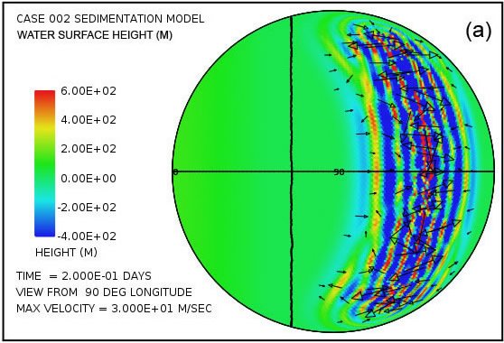
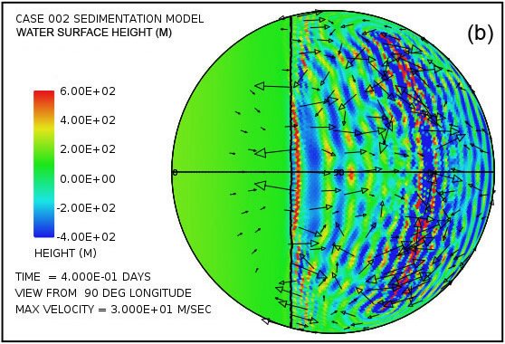
Fig. 2. Plots of water surface height at (a) 4.8 hrs and (b) 9.6 hrs after the beginning of a calculation in which the locking and sudden release of subduction zone fault segments located along the meridian at 126° longitude in the deep ocean generates a train of large-amplitude tsunami waves that begin to invade a circular supercontinent centered at 0° latitude and 0° longitude, located to the left of the heavy vertical line. Water surface height is relative to the mean sea level.

Other distributions of subduction zone were examined, including a single zone along the meridian at 180° longitude, and also a single zone along the equator from 90° to 270° longitude. The other distributions gave qualitatively similar results as those of the illustrative cases presented below.

An Illustrative Case

To illustrate the global sediment patterns we choose a simple geometry of a single circular continent, centered at the equator and zero degrees longitude, covering 38% of the earth’s surface. The ocean bottom surrounding the continent is taken to have a uniform height of –4000 m (–13,123 ft) relative to the mean sea level. The height of the continent at its center is 100 m (328 ft) relative to mean sea level and smoothly decreases to –72 m (–236 ft) at its edge. Initially the water is at rest with its surface at sea level. The continent surface is assumed everywhere to consist of crystalline bedrock. The earth is assumed to be spinning at its current rate of rotation.

An astonishing feature in the pattern of water flow emerges very early in the calculation with this model. Fig. 3 shows the water surface height at times of 2.5 and 5.0 days as viewed from four points 90° apart above the equator. Especially surprising is the remarkable elevation of the water surface height relative to sea level above most of the continent as Fig. 3(a) and Fig. 3(b) reveal. The greatest elevation of the water surface occurs within the large anti-cyclonic gyres in the pattern of water flow at high latitudes. These gyres are analogous to the high-pressure circulations (highs) at mid and high latitudes in the atmosphere, systems that rotate counterclockwise in the northern hemisphere and clockwise in the southern. The steady accumulation of water on the continent surface—at least until a state of equilibrium can be reached—is a consequence of the tsunamis carrying water onto the continent at a higher rate than can drain away back into the ocean through the influence of gravity. The anti-cyclonic gyres are the consequence of the Coriolis effect that contributes a force perpendicular to the direction of the water flow, that is, toward the center of the gyre (the –fk × u term in Eq. A14). This force acts to balance the pressure gradient force that acts in the direction outward from the center of the gyre (the g∇ h^† term in Eq. A14) due to the height of the water there. The magnitude of the Coriolis effect, which varies with the sine of the latitude, is zero at the equator and maximum at the poles. In this example, the Coriolis effect clearly exerts a major influence on the overall pattern of water flow above the continental surface.

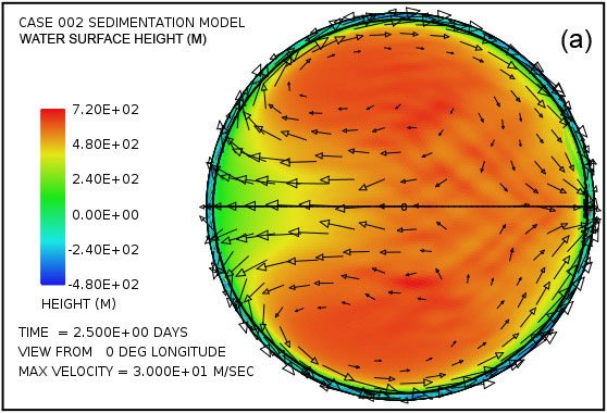
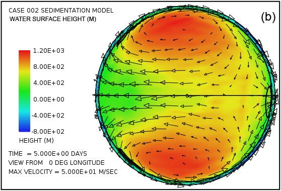
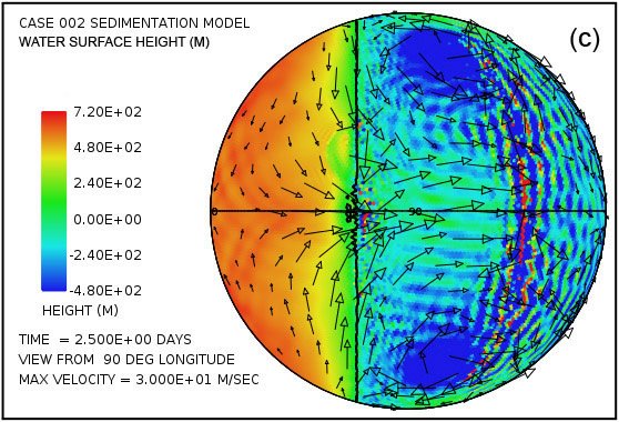
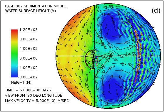
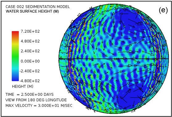
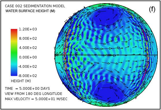
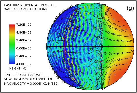
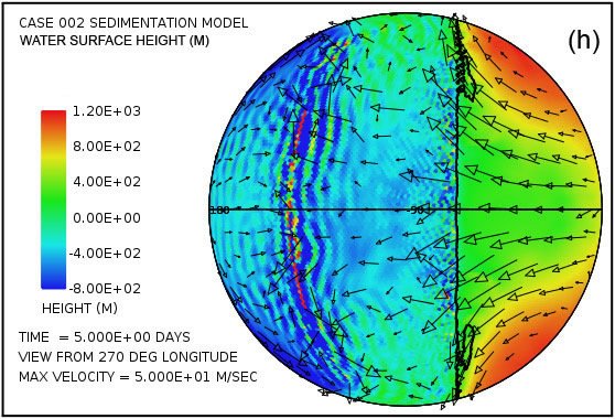
Fig. 3. Plots (in color) of water surface height at times of 2.5 days (a, c, e, g) and 5.0 days (b, d, f, h) viewed at 90° intervals of longitude above the equator. Arrows denote velocity of the water column. Note that the height scales and velocity scales differ between the two times. Surface height is relative to the mean sea level. Note the significant water surface height above the continental surface.

Moreover, plots in Fig. 3(c)–(f) reveal that four strong cyclonic gyres also arise at higher latitudes in the oceanic hemisphere. These gyres, analogous to low-pressure systems in the atmosphere, rotate in the clockwise direction in the northern hemisphere and in the counterclockwise direction in the southern hemisphere. In this calculation, they are associated with a significant depression of the ocean surface. At five days, as indicated in plots (d) and (f), this lowering of the ocean surface at the centers of the gyres exceeds 1000 m (3280 ft) below the mean sea level.

At the time of five days the flow pattern is approaching the condition at which the amount of water emplaced on the continent by the tsunamis is balanced by runoff from the elevated water levels on the continent. Because the Coriolis effect is smaller at low latitudes, most of the runoff occurs at these lower latitudes, as is evident in Fig. 3. This runoff also results in noticeable bedrock erosion, as the black contour line denoting a continent surface elevation of –300 m (–984 ft) indicates in plots (d) and (h). The general flow pattern established by the time of five days was found to persist throughout the 150-day period assumed for the interval in which the waters prevailed during the Flood.

Fig. 3 also displays the sort of water column velocities that arise above the continent surface. In the plots at five days, the plotted column velocities have been limited in amplitude to 50 m/s. Using the criteria for fluid turbulence developed above, one finds that the water depths and water column velocities imply that essentially everywhere over the continent the flow is in the strongly turbulent regime. It therefore has the ability to transport a considerable sediment load. Over much of the continent, especially along its margins, the velocity at the base of the water column significantly exceeds the cavitation threshold velocity and hence significant erosion is implied. Sediment produced from bedrock erosion is readily suspended in the turbulent flow. Wherever the sediment load exceeds 10% by volume in the basal layer, sediment deposition occurs. Once a sediment layer is present, it is vulnerable to being eroded, suspended, and transported before being redeposited elsewhere. Bedrock erosion and sediment deposition generate topographical relief on the continental surface, relief that also affects the pattern of water flow.

Fig. 4 attempts to provide an overview of erosion, transport and sedimentation that unfolds over a span of 100 days in this model. It uses pairs snapshots, at times of 50 and 100 days, showing by means of color, respectively, (i) the water surface height above initial sea level, (ii) the water depth, (iii) the cumulative bedrock erosion, (iv) the instantaneous thickness of sediment suspended by the turbulent flow, (v) the net cumulative amount of sediment remaining on the surface as a result of the ongoing processes of deposition and erosion, and (vi) the topography of the continental surface as erosion and deposition and isostatic compensation jointly act to alter it. Arrows in all the plots in Fig. 4 represent the water velocities at the bottom of the water column just above the land surface. For better clarity, water speeds have been clipped at 30 m/s. For reference, the water speed for the onset of cavitation is 15 m/s. The vigorous and highly turbulent water flow, whose energy is maintained by the tsunamis, is sufficient to suspend more than 150 m (492 ft) of sediment near the centers of the circular flow patterns at the high latitudes and several tens of meters most other places above the continent as indicated in Fig. 4(g). As the depths of deposited sediment become large beyond 50 days, the amount of suspended sediment diminishes, as observed in Fig. 4(h). Nevertheless, the turbulent water transports staggering volumes of eroded sediment for thousands of kilometers across the continent surface.

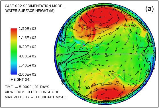
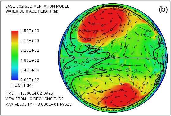
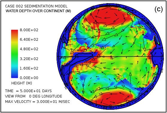
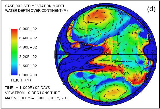
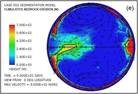
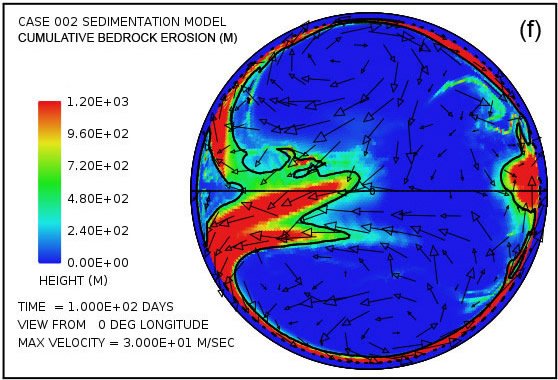
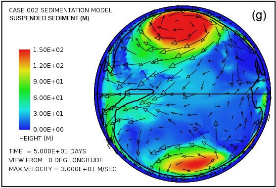
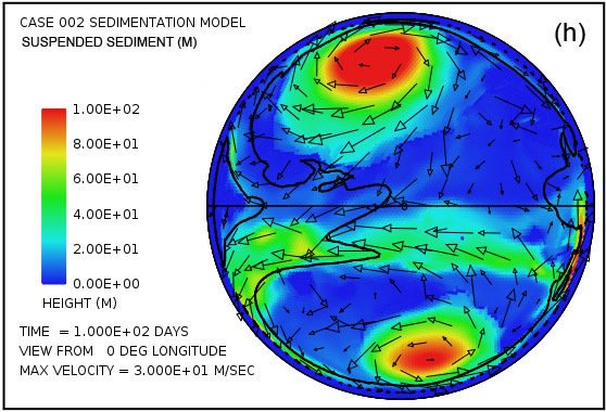
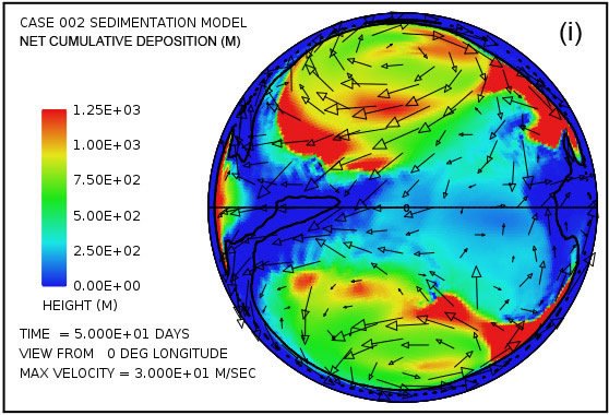
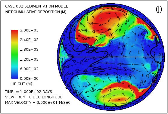
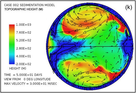
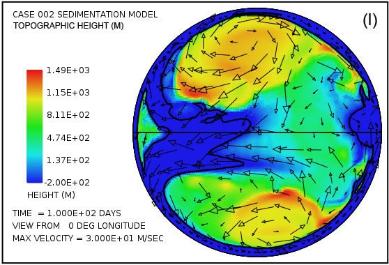
Fig. 4. Snapshots at 50 and 100 days of the water surface height above sea level (a, b); the water depth above the continent (c, d); the cumulative bedrock erosion (e, f); the instantaneous thickness of sediment suspended by the turbulent flow (g, h); the net amount of sediment on the surface as a result of deposition and erosion (i, j); and the topography of the continental surface (k, l). Arrows represent the water velocity just above the land surface that is used in the erosion submodel.

Plots (a) and (b) of Fig. 4 show that the astonishing flooding of the continental surface observed at 5 days in Fig. 3 persists to 100 days. The water surface height exceeds 1500 m (4921 ft) above the mean sea level in the high-latitude anti-cyclonic gyres and generally exceeds 500 m (1640 ft) above the mean sea level elsewhere. In contrast to plots in Figs. 4(a) and (b) which display water surface height, plots in Figs. 4(c) and (d) display the actual water depth down to the continent surface. Where that surface is below mean sea level, the water depth is set to zero. In other words, these plots display the water depth only where the land surface is above sea level. There are several noteworthy features in Fig. 4(c) and (d). First, while water depths are appreciable near the center of the gyres at 50 days, these regions have significantly been filled with sediment by 100 days such that the water depths there are noticeably smaller. Second, along margins of the gyres there are zones of very shallow water. As can be verified in Figs. 4(i) and (j), these are zones of thick sediment deposition. These zones represent regions where the land surface could have been exposed at various times during the cataclysm. In addition to the zones along the margins of the gyres, there are isolated dome-shaped spots that may have become what are referred to today as sedimentary basins. Two such spots are evident in Fig. 4(i) at approximately –30° latitude and –15° and –30° longitude. Both are on the order of a few hundreds of kilometers in diameter. After the Flood the excess weight of these huge mounds of sediment would have depressed both the crustal surface beneath them as well as the underlying mantle.

Plots in Figs. 4(e) and (f) reveal that most of the bedrock erosion occurs along the continent margin. Since in the cavitation model the erosion rate varies as the sixth power of the difference between the water speed and the cavitation onset speed, it is not surprising for erosion to be most intense at the continental margin where the tsunamis encounter an abrupt decrease in water depth and water speed increases dramatically. The contour line along the perimeter of the continent marks the depth of 300 m (984 ft) below sea level. Note that the most intense erosion is oceanward of this –300 m (–984 ft) contour line. The cumulative volume of bedrock erosion is enough to cover the surface of the entire continent with sediment to a mean depth of 670 m (2198 ft) after 50 days and 1109 m (3638 ft) after 100 days, reflecting an average erosion (and deposition) rate over 100 days of about 11 m/day.

Plots in Figs. 4(g) and (h) show the amounts of sediment suspended by the turbulent water. The average over the whole continent surface is 49 m (160 ft) at 50 days and 26 m (85 ft) at 100 days. The largest amounts are near the centers of the gyres where the depth of the water column is greatest. Plots in Figs. 4(i) and (j) display the cumulative net result of sediment deposition and sediment erosion. Plots in Figs. 4(k) and (l) reveal how the continent topography is altered by the processes of erosion, sediment transportation, sediment deposition, and partial isostatic adjustment. The amount of isostatic adjustment may be estimated by comparing the plots in Fig. 4 of cumulative erosion (e, f) and of net cumulative sedimentation (i, j) with the resulting topographic expression (k, l).

Noteworthy is the effectiveness of the tsunamis and the associated water dynamics to emplace hundreds of meters of sediment on top of the continent, above the mean sea level. If Genesis 7:24 which states, “And the water prevailed upon the earth one hundred and fifty days,” implies that the primary sedimentation of the Flood spanned 150 days, then an average sedimentation rate of 12 m/day (39.3 ft/day) over that interval accounts for the roughly 1800 m (5905 ft) of sediment on average residing presently on the continents. The average rates obtained in this illustrative calculation then are not too far from the average value inferred from the Genesis text.

Fig. 5 provides a more detailed picture of the suspended and deposited sediment when separated into the three assumed sediment classes. As mentioned earlier we assume that the erosional processes, especially cavitation, reduce crystalline bedrock into a mixture of relatively fine particles, 70% with a mean diameter of 0.063 mm (0.0025 in) corresponding to that of fine sand, 20% with a mean diameter of 0.25 mm (0.010 in) corresponding to medium sand, and 10% with a mean diameter of 1 mm (0.039 in) corresponding to coarse sand. Fig. 5 displays the lateral distribution of suspended sediment for each of these size classes at a time of 50 days. It also shows the lateral distribution of the deposited sediment by size class at this same time. The coarse sand has a much higher settling velocity than the fine and medium sand. It is therefore more difficult to maintain in suspension, as Fig. 5(e) reveals. It is also the first to fall from suspension as the flow velocity decreases. The coarse sand therefore tends to be deposited closer to its source as indicated in Fig. 5(f).

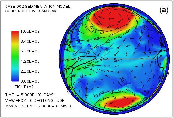
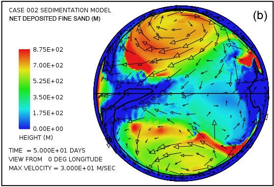
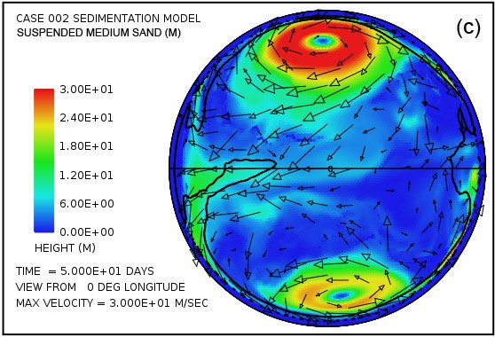
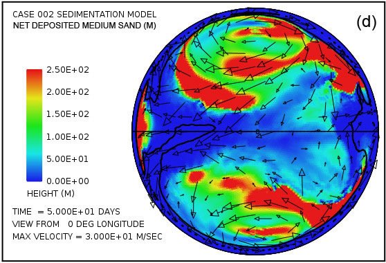
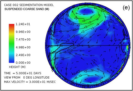
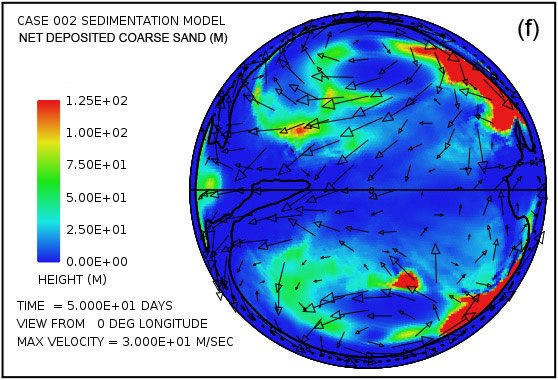
Fig. 5. Snapshot at a time of 50 days from the illustrative case: (a) suspended fine sand; (c) suspended medium sand; (e) suspended coarse sand; (b) cumulative deposited fine sand; (d) cumulative deposited medium sand; (f) cumulative deposited coarse sand. Amplitudes of the plots are scaled to match the 70:20:10 volume ratios produced by bedrock erosion for the three particle size classes.

A Second Illustrative Case

The case just described used a continent distribution consisting of a single spherical cap, centered at the equator, which covered 38% of the area of the globe. To add a bit more realism a second case is presented, one that preserves the parameter values of the first case but instead of a circular cap uses a Pangean-like continent distribution. Fig. 6 displays snapshots at 50 and 100 days of the water surface height relative to nominal (initial) sea level (a, b); water depth (c, d); cumulative bedrock erosion (e, f); instantaneous thickness of sediment suspended by the turbulent flow suspended (g, h); net cumulative deposition of sediment (i, j); and the topography of the continental surface as erosion and deposition and isostatic compensation jointly act to alter it (k, l). Arrows denote the mean water column velocity in (a, b) and water velocity at the base of the water column in (c–l).

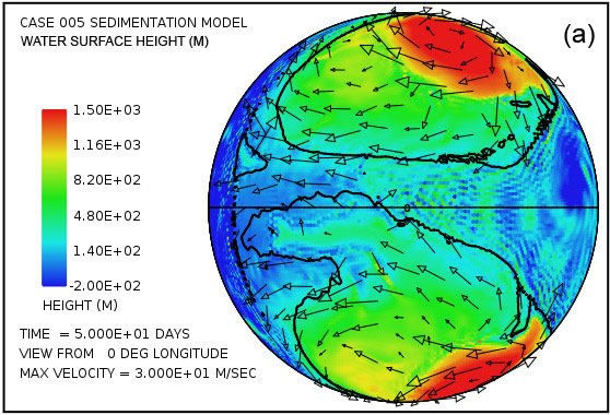
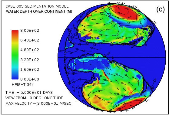
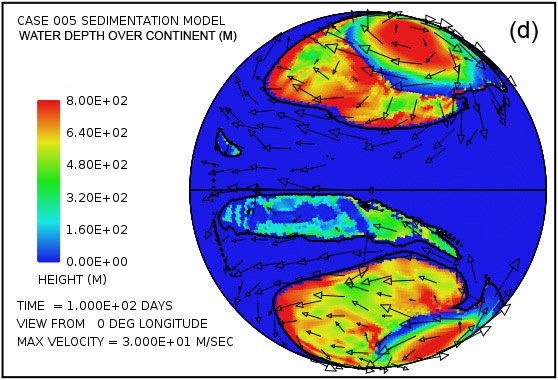
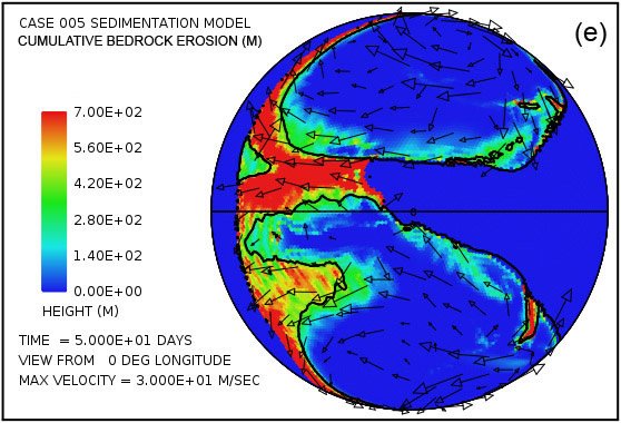
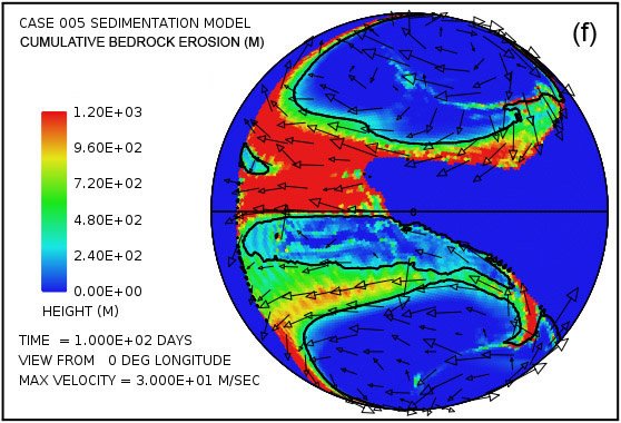
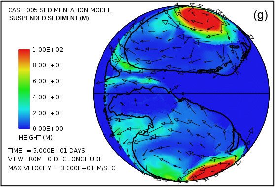
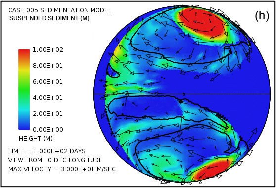
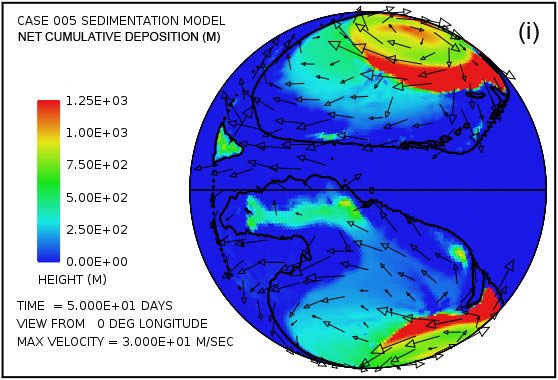
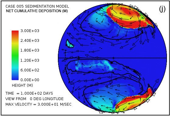
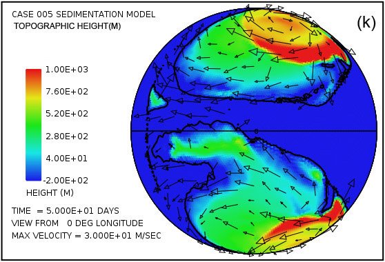
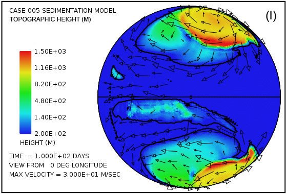
Fig. 6. Snapshots at 50 and 100 days from a case with a Pangean-like continent distribution. Colors denote water surface height above sea level (a, b); water depth above the continental surface (c, d); cumulative bedrock erosion (e, f); instantaneous thickness of sediment suspended by the turbulent flow (g, h); net amount of sediment on the surface as a result of deposition and erosion (i, j); and topography of the continental surface (k, l). Arrows denote mean water column velocity in (a, b) and water velocity at the base of the water column in (c–l).

This second illustrative case displays the same noteworthy features of the first case including the elevated water levels over the continent, especially within the prominent anti-cyclonic gyres at high latitudes and erosion concentrated along the continental margins. The cumulative volume of bedrock erosion is enough to cover the surface of the entire continent with sediment to a mean depth of 489 m (1604 ft) after 50 days and 878 m (2880 ft) after 100 days, reflecting an average rate over the 50 days of 9.8 m/day (31.4 ft/day). This case demonstrates hundreds of meters of sediment emplaced above sea level on top of the continental surface which initially itself was mostly above sea level.

Discussion

In the context of a reasoned defense of the Genesis Flood there are several major features of the earth’s continental surface that cry out for explanation. First is the sheer volume of fossil-bearing sedimentary rock present there today. The volume is sufficient to cover the continental surface to an average depth of about 1800 m or about 1.1 mi. What was the source of this massive volume of sediment during the Flood’s short time span? Second is the location of this huge volume of sediment. It occurs on top of the continents, whose surface generally lies above sea level. This raises the question, what sort of water process might conceivably emplace so much sediment above sea level on top of the land surface? A third issue has to do with the internal depositional characteristics of the sediment. Generally speaking, most of the sediment occurs as a vertical succession of horizontal layers, often with vast lateral extent. Such an orderly layer-cake pattern of laterally extensive strata is readily observed, for example, for the sediments exposed in the walls of the Grand Canyon. What sort of transport and depositional process could conceivably generate such uniform layers over such vast horizontal distances?

A fourth prominent feature of the earth’s surface includes the so-called continental shields, including the Canadian, Baltic, Angaran (Siberian), African, Indian, Australian, and Antarctic shields. These large areas of exposed Precambrian crystalline igneous and high-grade metamorphic rocks have experienced significant erosion (often with more than 1 km (0.62 mi) of crystalline rock removed), are nearly flat, and have negligible, if any, sediment cover. When in earth history did such intense erosion occur if it was not during the Genesis Flood? And by what sort of process?

A fifth noteworthy feature is the phenomenon of so-called sedimentary basins that cover much of the non-shield portions of the continent surface. These basins are commonly described by the standard earth science community as regions of long-term subsidence that have provided accommodation space for infilling by sediments. Frequently absent from the discussion of most basins is the mechanism responsible for their subsidence. Basin sediments almost invariably have notably lower densities than the basement rocks beneath. Within stable craton interiors there is no obvious reason why lower density rock at the surface should displace higher density rock at depth to yield subsidence. Because a convincing mechanism for subsidence has not been forthcoming in so many contexts, this issue continues to be regarded as a topic in need of further study within the earth science community.

This numerical investigation appears to shed at least some new light on all five of these important issues. First, in regard to a source for the huge volume of Phanerozoic sediment present in the continental rock record, the numerical study reveals that tsunami-driven cavitation erosion during the time span of the Flood can generate new sediment at a rate sufficient to account for a sizable fraction of the Phanerozoic sediment inventory. The cavitation, occurring at water speeds of several tens of m/s, rapidly reduces crystalline continental crustal rock to sand-sized and smaller particles.

Moreover, the existence of so many shield areas today testifies to the reality of extreme erosion of the igneous bedrock over vast portions of today’s continents. These shield areas are remarkably flat with little or no erosional channeling and generally display little or no sedimentary deposition subsequent to their intense erosional beveling. In the context of the Flood, these areas would seem to be obvious candidates as source areas for at least some of the sediment we find elsewhere on the continental surface. A major issue, however, is an erosional mechanism sufficiently potent to erode such hard crystalline rock to depths of up to a kilometer or more within the time span of the Flood and also to do so in such a uniform manner across such laterally extensive areas. The frequent, large-amplitude tsunamis in this numerical model appear adequate for such a task. Indeed, it is difficult to imagine an alternative mechanism capable of accomplishing such intense and laterally extensive erosion to produce a surface with such astonishing flatness.

In regard to an explanation for why so much sediment is emplaced on top of the continents when their surfaces mostly lie above sea level, this numerical model also provides especially helpful insight. The short answer is that the tsunamis initially bring more water onto the continent surface than can drain via gravity back into the ocean basin. The water level therefore rises over the continent surface until the water height is sufficient for the runoff rate to match the emplacement rate from the tsunamis. Remarkably, in the illustrative cases, the resulting average water depth is many hundreds of meters, with maximum values exceeding 1500 m (4921 ft) that occur at the centers of anti-cyclonic gyres at high latitudes in both northern and southern hemispheres. These gyres are expressions of the Coriolis effect caused by the earth’s rotation. The gyres serve to organize the overall water motions over the continent regions into a notably smooth and coherent pattern of flow. The water speeds and depths are sufficient to sustain the level of turbulence needed to suspend the large volume rate of sediment produced by cavitational erosion, to transport it to distant locations, and to deposit that sediment in thicknesses reaching hundreds to thousands of meters over much of the continental surface. The tsunami-driven flow accounts not only for erosion of significant volumes of sediment but also its emplacement above sea level on top of the continents in coherent patterns with large lateral dimensions and thicknesses in excess of a kilometer. The model thus seems to account for the emplacement of the sediment on top of the continental surface and also for some aspects of its internal character.

In regard to the internal character of the sedimentary deposits themselves, the horizontal spacing of about 120 km (74.5 mi) between grid points in the computational grid for this global model severely limits the sort of structural detail that can be resolved at the local scale within individual sediment layers. Certainly there is observational evidence for long runout underwater debris flows, apparently driven by gravity, such as the one which generated the Whitmore Nautiloid Bed in Arizona and Nevada. Such observations have drawn attention to the issue of the primary sediment transport mechanism during the Flood, specifically whether the transport was primarily by gravity driven debris flows or by sediment suspended in a thick column of rapidly moving turbulent water. Although it is beyond the scope of what is feasible to discuss here, the calculations in this paper show that the sediment concentrations frequently tend to become large, even to the point of hyper-concentrated flow at the base of the turbulent water column. In such cases, it appears that it might become difficult to distinguish whether the dense sediment is being moved by gravity or via drag from above. Assuredly, this issue deserves more detailed study in the future.

An important result of this investigation is that the tsunami mechanism provides a simple to understand explanation for the runoff of the Flood water from the continental surface. As the gravitational potential energy from the sinking lithospheric slabs and rising mantle plumes which had been driving the runaway motions begin to be significantly depleted, the surface plate speeds begin to diminish, the tsunamis begin to decrease in frequency and in amplitude, the flow rates of the water currents on the continents start to fall, and the water that had been emplaced and maintained over the continental surface to such great depths begins to drain back into the ocean basin. The time frame of Genesis 8 indicates that the runoff required about five months. Hence the model also addresses the commonly asked questions as to the source of the Flood waters and where these waters went after the Flood.

The numerical calculations in addition provide a possible explanation for the so-called sedimentary basins. As mentioned in Appendix F, it was found early in the testing the model that sediment thicknesses of several hundreds of meters routinely arise. When such large thicknesses were allowed to augment the original continent topography with no isostatic compensation whatsoever, a type of numerical instability emerged. The unstable behavior involved the formation of localized mounds of sediment, typically a few hundred kilometers across and hundreds of meters high. This topography, in turn, forced the water flow to become concentrated in channels between these sediment mounds and for enhanced deposition to occur on top of the mounds where the flow depths and velocities were small. The higher the mounds grew, the stronger this tendency became. A simple remedy for this problem was to include partial isostatic compensation to allow the basement to subside in response to the sediment load above it. The scheme described in Appendix F alleviates this instability. The mounds of sediment nevertheless still arise but with reduced amplitude. This behavior observed in the numerical model suggests a simple and straightforward explanation for the subsidence associated with what are today referred to as sedimentary basins. The explanation is that the sediments now found in these so-called basins correspond to large piles of sediment deposited on the continental surface during the Flood by the large-scale turbulent water processes. The weight of these mounds of sediments has subsequently depressed the original surface beneath the sediments into its present basin-like profile.

A notable feature of the computational results is the significant depth of the water over much if not most of the continental surface sustained by frequent large-amplitude tsunamis. Among the issues this raises are observations such as animal trackways, which indicate some portions of the land surface were above water. It is noteworthy that in the illustrative cases after about 50 days the topographic elevation of some of the sediment mounds brings them some of the time above the water surface. This is consistent with the fact that evidences for land surface exposure within the Paleozoic portion of the sediment record, that is, during the earlier part of the Flood, are scant, while such evidences become more and more common through the Mesozoic and Cenozoic parts of the record, that is, during the Flood’s latter stages. This feature of high water levels over most of the continental area during most of the depositional stage of the Flood also has bearing on the issue of where the plants and animals buried in later Flood sediments were being warehoused during the earlier stages of the Flood. The illustrative cases described in this paper would seem to imply that they were either floating at the water surface or were being persistently suspended by the highly turbulent flow. Another possibility not addressed in the illustrative cases, however, is that there were pre-Flood continental regions with high topography which were not flooded until later into the Flood. The illustrative cases used initially smooth continental surfaces whose maximum elevation above nominal sea level was only about 100 m (328 ft). Clearly this issue deserves further study in the future.

A crucial aspect of the model that also invites further scrutiny is the locking/slipping mechanics of subducting lithosphere responsible in the model for generating the large-amplitude tsunamis. Plate speeds during the Flood, as constrained by the timescale of Genesis chapters 7 and 8 and the widths of new ocean floor generated, must have been at least 108 times higher than is typical today. On the other hand, as discussed in Appendix F, the strength of mantle rock and possibly also much of the lithosphere was reduced by a similar factor. It is therefore difficult to extrapolate with any degree of confidence today’s subduction zone mechanics to the state of affairs that prevailed during the Flood. In today’s world, the subducting slab and the overriding plate are always locked, except for brief episodes lasting from seconds to minutes, during which rapid slip occurs, resulting in earthquakes and sometimes large tsunamis. The time between slip events on many subduction zone segments today is measured in terms of centuries. A horizontal speed of 10 cm/yr for one of the plates with the other plate fixed, for example, implies 10 m (32.8 ft) of slip between plates every 100 years or 20 m (65.6 ft) of slip every 200 years. How this process might have operated during the Flood when plate speeds were dramatically higher is far from clear. The key issue would seem to be the amount of stress the fault between the plates could sustain without slip occurring. It may well be that the strength reduction due to the runaway process may have affected the lithosphere less than the mantle beneath and allowed relatively higher levels of stress in the locked plates and consequently larger surface deflections between episodes of slip. Further careful study, likely utilizing numerical tools, is urgently needed for this vital issue.

It is to be emphasized that the two illustrative cases presented in this paper are highly simplistic relative to the real earth and the full suite of processes that played a role during the Flood. One of the more glaring deficiencies is that in both cases the continent configuration remained constant, with no continental breakup and no subsequent motion of the component blocks. Allowing the initial continent configuration to break apart and the resulting blocks to migrate almost certainly will result in major changes in patterns of water flow, erosion, and sedimentation. Moreover, neither of the two cases included any initial topography apart from a slightly domed continent surface. Neither included any dynamic topography arising from flow of rock inside the mantle. Such variations in continent surface height can reach several kilometers in amplitude, especially when subduction is occurring near a continental margin.

Furthermore, neither calculation included any changes at all in the location or activity of the subduction zones. Temporal changes in where the tsunamis are generated and their amplitude undoubtedly affect the patterns of water flow, erosion, and sedimentation. Neither of the two cases included any temporal or spatial changes in the height of the ocean bottom, nor any easily eroded sediment present initially on the continental surface, nor any motions of the deposited sediments due to gravity-driven debris slides, nor any contributions to bedrock erosion from plucking or suspended load abrasion, nor any of a much longer list of processes that undoubtedly affected the sediment distribution in notable ways. In other words, the numerical model described here is merely a beginning, primitive framework for treating the water flow, erosion, and sedimentation of the Flood on a global scale. It is one, however, that has the flexibility to be augmented to address most of the issues just mentioned.

Yet even this beginning framework is yielding important new insights. The finding that large-amplitude tsunamis produced by locking and episodic unlocking of subducting ocean plates into the mantle during the Flood can cause significant depths of water spontaneously to accumulate over the continental interior represents a notable discovery. One of the greatest unresolved issues concerning the Genesis Flood has been the mechanism by which the entire continental surface could possibly be flooded with water. A companion issue has been the mechanism responsible for the draining away of this water. The steady slowing of tsunami generation due to exhaustion of the gravitational energy driving the rock motions in the mantle during the waning stages of the Flood causes the water velocities steadily to drop to zero and the water to drain from the continent. Both issues are resolved utilizing only the inventory of water presently in the world’s ocean basins. These mechanisms possibly might never have been identified apart from numerical simulation experiments such as these.

The version of this model presented at the 2013 International Conference on Creationism (Baumgardner 2013) utilized an entirely different mechanism for driving the water motions. In that case the mechanism involved several near approaches with the earth of a moon-sized body that raised large-amplitude tides. That paper suggested that six such near encounters spaced about 30 days apart might plausibly account for the six megasequences so prominent in the sediment record and the nearly global erosional unconformities associated with them (Sloss 1963). In view of the results presented in this paper, one might wonder whether these more recent findings supersede or even negate the earlier ones. It is the author’s opinion that the two papers and the two forcing mechanisms are mutually compatible. To me it is at least conceivable that both mechanisms might have operated during the Flood. However, the tsunami mechanism—occurring as a direct consequence of the rapid plate tectonics that logically must have taken place during the Flood—in my view is vastly more likely. Especially because the tsunami mechanism appears to account so readily for the flooding of the continental regions during the Flood and for the runoff in its latter stages, I believe it deserves significant further attention. The scenario of a near approach with earth by a moon-sized body described in the 2013 paper was, quite candidly, a near desperation effort on my part to identify an adequate mechanism for driving the water flow. Were it not for the conceivable ability of this scenario to account for the megasequences, I doubt that I would have a sufficient level of interest to pursue it any further.

Conclusion

Numerical simulation offers a means for investigating phenomena that are impossible, either because of their physical scale or the extreme conditions they entail, or both, to explore experimentally in a repeatable manner in the laboratory. The Genesis Flood certainly falls into this category. This paper describes a beginning attempt to apply known physical laws, physical processes that can be investigated in the laboratory, and processes on larger scales that can be studied and characterized by measurements in the present, to model important aspects of this unique cataclysmic event. The numerical model exploits the shallow water approximation to represent water flow in a thin layer on the surface of a rotating sphere corresponding to the earth. It utilizes the theory of open-channel flow to treat the suspension and transport of sediment by turbulent flowing water. As its mechanism for erosion it utilizes cavitation. To drive the water flow it draws upon a currently observable consequence of plate tectonics, namely, the locking and sudden release of a subducting lithospheric plate along its fault contact with the overriding plate in a subduction zone. Today, when a subducting plate unlocks and rebounds, the upward motion of the plate can, and often does, generate a water wave known as a tsunami. During the Flood, when plate speeds were orders of magnitude higher than they are today, the amplitudes of the tsunamis may conceivably have been vastly larger.

In the numerical model such large-amplitude tsunamis drive the global water flow. These tsunamis, astonishingly, inundate the continental regions everywhere with many hundreds of meters of water. The tsunamis initially emplace water on the continent faster than it can run off under the influence of gravity. Equilibrium between water emplacement and runoff occurs only after water over the continental surface reaches depths of many hundreds of meters. In the meantime, water speeds along the continental margins quickly exceed the cavitation threshold, leading to intense erosion there of the continental bedrock. The Coriolis effect caused by the earth’s rotation leads to large, mostly stationary, circulation patterns at high latitudes above the continental regions in both northern and southern hemispheres. The persisting large-scale flow of turbulent water transports the eroded sediment and deposits it in a pattern characterized by large spatial scales. When plate speeds begin to fall due to the exhaustion of gravitational energy driving the motion in the mantle, the tsunamis decrease in frequency and in amplitude, water velocities drop toward zero, and the water that had been standing hundreds of meters deep over the continental surface drains back into the ocean basin. In the two illustrative examples, the erosion and deposition rates approach those needed to account for the 1800 m (5905 ft) of sediment on average that blankets today’s continental surface.

This numerical model, basic as it is, sheds new light on several important issues relating the Flood. It seems to account (1) for how the continents, which today are mostly above sea level, were deeply inundated during the Flood; (2) for the source of the water responsible for the inundation; and (3) for where all that water went at the end of the Flood. It appears to account (4) for how such a huge volume of new sediment could arise during the short time span of the Flood; (5) for how the astonishingly thick sediment sequences we observe in the sediment record managed to be deposited on top of the normally high-standing continents; and (6) for the vast lateral scales and horizontal continuity of many if not most individual layers within the sediment sequence. It appears to account (7) for the vast regions of flat, deeply beveled Precambrian basement rock known as continental shields. Finally, it may well account (8) for how sedimentary basins came into being.

These promising results invite several future refinements and additions. Examples include augmenting the model to treat continental breakup, motions of the resulting continental blocks, migration of subduction zones, and dynamic topography rising from movement of rock inside the mantle. Such refinements almost certainly will lead to additional insights concerning this cataclysm that in Noah’s day so dramatically altered the face of the earth. My prayer is that improved understanding of the processes that generated the fossil-bearing sediment record during the Flood might strengthen the confidence of many in the historical reliability of Genesis 1–11, and hence their confidence in the entirety of Scripture, and thereby strengthen their loyalty and devotion to the Lord Jesus.

References

Ager, D. V. 1973. The Nature of the Stratigraphical Record. London, United Kingdom: MacMillan.

Apsley, D. D. 2009. “Structure of a Turbulent Boundary Layer” (lecture notes from course entitled “Turbulent Boundary Layers,” Manchester University, United Kingdom). http:// personalpages.manchester.ac.uk/staff/david.d.apsley/ lectures/turbbl/regions.pdf.

Arndt, R. E. A. 1981. “Cavitation in Fluid Machinery and Hydraulic Structures.” Annual Reviews of Fluid Mechanics 13: 273–328.

Austin, S. A. ed. 1994. Grand Canyon: Monument to Catastrophe. Santee, California: Institute for Creation Research.

Bagnold, R. A. 1966. “An Approach to the Sediment Transport Problem from General Physics.” Geological Survey Professional Paper 422-I, I1–I37. Washington, D.C: United States Government Printing Office.

Baker, V. 1974. “Erosional Forms and Processes from the Catastrophic Pleistocene Missoula Floods in Eastern Washington.” In Fluvial Geomorphology. Edited by M. Morisawa, 123–48. London, United Kingdom: Allen and Unwin.

Baumgardner, J. R. 2013. “Explaining the Continental Fossil- Bearing Sediment Record in Terms of the Genesis Flood: Insights from Numerical Modeling of Erosion, Sediment Transport, and Deposition Processes on a Global Scale.” In Proceedings of the Seventh International Conference on Creationism. Edited by M. Horstemeyer. Pittsburgh, Pennsylvania: Creation Science Fellowship, Inc. http:// media.wix.com/ugd/a704d4_70de439475d229ba9231b545d e57d670.pdf.

Baumgardner, J. R. 2003. “Catastrophic Plate Tectonics: The Physics Behind the Genesis Flood.” In Proceedings of the Fifth International Conference on Creationism. Edited by R. L. Ivey, Jr., 113–26. Pittsburgh, Pennsylvania: Creation Science Fellowship. http://media.wix.com/ugd/a704d4_ bfc60d3bb5aad292ce1e8d9384b9eb87.pdf.

Chanson, H. 1997. Air Bubble Entrainment in Free-Surface Turbulent Shear Flows. London, United Kingdom: Academic Press.

Darcy, H. 1857. Recherches Expérimentales Relatives au Mouvement de L’Eau dans les Tuyaux (Experimental Research Relative to the Movement of Water in Pipes). Paris, France: Mallet-Bachelier.

Falvey, H. T. 1990. “Cavitation in Chutes and Spillways.” Engineering Monograph No. 42. Denver, Colorado: U.S. Bureau of Reclamation.

Hagen, G. 1854. “Über den Einfluss der Temperatur auf die Bewegung des Wassers in Röhren” (“On the Influence of Temperature on the Motion of Water in Pipes”). Mathematische Abhandlungen der Koeniglichen Akademie der Wissenschaften zu Berlin: 17–98.

Harris, C. K. 2003. “Suspended Sediment Transport” (lecture notes from graduate course entitled “Sediment Transport Processes in Coastal Environments,” Virginia Institute of Marine Science).

Jiménez, J., and O. Madsen. 2003. “A Simple Formula to Estimate Settling Velocity of Natural Sediments.” Journal of Waterway, Port, Coastal, and Ocean Engineering 129 (2): 70–78.

Kolmogorov, A. N. (1941) 1991a. “The Local Structure of Turbulence in Incompressible Viscous Fluids at Very Large Reynolds Numbers.” Doklady Akademii Nauk SSSR 30: 299–303. Reprinted in Proceedings of the Royal Society of London, Series A 434: 9–13.

Kolmogorov, A. N. (1941) 1991b. “Dissipation of Energy in the Locally Isotropic Turbulence.” Doklady Akademii Nauk SSSR 32:19–21. Reprinted in Proceedings: Mathematical and Physical Sciences 434 (1890): 15–17.

Majewski, D., D. Liermann, P. Prohl, B. Ritter, M. Buchhold, T. Hanisch, G. Paul, W. Wergen, and J. Baumgardner. 2002. “The Global Icosahedral-Hexagonal Gridpoint Model GME: Description and High Resolution Tests.” Monthly Weather Review 130 (2): 319–38.

Momber, A. W. 2003. “Cavitation Damage to Geomaterials in a Flowing System.” Journal of Materials Science 38 (4): 747–57.

Murai, H., S. Nishi, S. Shimizu, Y. Murakami, Y. Hara, T. Kuroda, and S. Yaguchi. 1997. “Velocity Dependence of Cavitation Damage (Sheet-Type Cavitation).” Transactions of the Japan Society of Mechanical Engineers, Part B 63 (607): 750–56.

O’Connor, J. E. 1993. “Hydrology, Hydraulics, and Geomorphology of the Bonneville Flood.” Geological Society of America Special Paper 274.

Pope, S. B. 2000. Turbulent Flows. Cambridge, United Kingdom: Cambridge University Press.

Prandtl, L. 1905. “Über Flüssigkeitsbewegung bei sehr kleiner Reibung” (“On Fluid Flow with very little Friction”). Verhandlungen des Dritten Internationalen Mathematischen Kongresses, Heidelberg, 484–91. Leipzig, Germany: Teubner Verlag.

Prothero, D. R., and F. Schwab. 2004. Sedimentary Geology: An Introduction to Sedimentary Rocks and Stratigraphy. 2nd ed. New York, New York: W. H. Freeman.

Reynolds, O. 1883. “An Experimental Investigation of the Circumstances Which Determine Whether the Motion of Water Shall Be Direct or Sinuous, and of the Law of Resistance in Parallel Channels.” Philosophical Transactions of the Royal Society of London 174: 935–82.

Richardson, L. F. 1920. “The Supply of Energy from and to Atmospheric Eddies.” Proceedings of the Royal Society of London, Series A, 97 (686): 354–37.

Sloss, L. L. 1963. “Sequences in the Cratonic Interior of North America.” Geological Society of America Bulletin 74 (2): 93–113.

Staniforth, A., and J. Côté. 1991. “Semi-Lagrangian Integration Schemes for Atmospheric Models—A Review.” Monthly Weather Review 119: 2206–223.

Stokes, G. 1851. “On the Effect of the Internal Friction of Fluids on the Motion of Pendulums.” Transactions of the Cambridge Philosophical Society 9: 8–106.

Whipple, K. X., G. S. Hancock, and R. S. Anderson. 2000. “River Incision into Bedrock: Mechanics and Relative Efficacy of Plucking, Abrasion, and Cavitation.” Geological Society of America Bulletin 112 (1–2): 490–503.

Williamson, D. L., J. B. Drake, J. J. Hack, R. Jakob, and P. N. Swaztrauber. 1992. “A Standard Test Set for Numerical Approximations to the Shallow Water Equations in Spherical Geometry.” Journal of Computational Physics 102 (1): 211–24.

Winston, D., and P. K. Link, 1993. “Middle Proterozoic Rocks of Montana, Idaho, and Washington: The Belt Supergroup.” In Precambrian of the Conterminous United States. Edited by J. Reed, P. Simms, R. Houston, D. Rankin, P. Link, R. Van Schmus, and P. Bickford, 487–521. Boulder, Colorado: Geological Society of America, The Geology of North America, v. C-3.

Wohl, E. E. 1992. “Bedrock Benches and Boulder Bars: Floods in the Burdekin Gorge of Australia.” Geological Society of America Bulletin 104 (6): 770–78.

Appendix A: What Is Fluid Turbulence?

The importance of the role of turbulence in fluids was clearly recognized in the early part of the 19th century when the pressure drop in water pipes and the drag of water on ships were hydraulics issues of considerable practical concern. It was known that both the pressure drop in pipes and the drag exerted on ships as they moved through the water had two components, one linear and the other approximately quadratic in the fluid velocity. Surprisingly, it was found that only the first one depended on the viscosity of the fluid. In the 1850s G. Hagen and H. Darcy both published careful measurements of fluid flow through large pipes. They both noted that the quadratic component was associated with disordered motion in the fluid and that it became the dominant contribution when the pipes were large and the flow speed became sufficiently high. They speculated that the increased drag was due to the energy spent in creating velocity fluctuations as the flow became turbulent.

G. Stokes (1851) was the first to show that the onset of turbulent flow depends on the ratio of the inertial force of the moving fluid to the viscous forces acting upon it. This ratio is today known as the Reynolds number, named after O. Reynolds, who in the 1870s and 1880s published a series of papers describing results of his careful experimental studies on the transition from laminar to turbulent fluid flow, first in pipes and then in other settings. Reynolds, in an 1883 paper (Reynolds 1883), stressed the importance of this dimensionless ratio that now bears his name. This ratio, the Reynolds number Re, is usually expressed as Re = uL/ν, where u is the fluid velocity, L is a characteristic spatial dimension of the flow, and ν is the kinematic viscosity.

In the early 20th century Ludwig Prandtl made an important computational advance by introducing the concept of a fluid boundary layer. In a groundbreaking 1905 paper he showed that the equations for fluid flow could be simplified by dividing the flow field into two regions: a boundary layer in which the fluid viscosity plays a major role and the region outside the boundary layer, where the viscosity can be neglected with no significant effects on the solution. Prandtl’s boundary layer theory provided crucial new understanding of skin friction drag and how streamlining reduces drag on airplane wings and other bodies that move relative to a fluid environment.

But what is fluid turbulence? The British scientist L. F. Richardson (1920) described fluid turbulence in poetic fashion as follows:

Big whorls have little whorls
That feed on their velocity,
And little whorls have lesser whorls
And so on to viscosity.

Richardson’s picture of turbulence is a flow comprised of a hierarchy of vortices, or eddies, from large to tiny. These eddies, including the large ones, are unstable. The shear that their rotation exerts on the surrounding fluid generates smaller new eddies. The kinetic energy of the large eddies is thereby passed to the smaller eddies that arise from them. These smaller eddies in turn undergo the same process, giving rise to even smaller eddies that inherit the energy of their predecessors, and so on. In this way, the energy is passed down from the large scales of motion to smaller and smaller scales until reaching a length scale sufficiently small that the molecular viscosity of the fluid transforms the kinetic energy of these tiniest eddies into heat.

In 1941, the Russian A. N. Kolmogorov (1991a, b) postulated that for very high Reynolds numbers, the small scale turbulent motions are statistically isotropic (i.e., have no preferential spatial direction). In general, the largest scales of a flow are not isotropic, since they are determined by the particular geometrical features of the problem. Kolmogorov’s idea was that, in the energy cascade which Richardson described, this geometrical and directional information at the largest scale is lost. This means that the statistics of the smaller scales has a universal character and that they are the same for all turbulent flows when the Reynolds number is sufficiently high. He further hypothesized that for very high Reynolds numbers the statistics of small scales are universally and uniquely determined by the viscosity ν and the rate of energy dissipation ε. With only these two parameters, a unique length λ can be obtained by dimensional analysis given by λ = (v₃/ε)_¼. This is today known as the Kolmogorov length scale.

Kolmogorov’s concept was that turbulent flow is characterized by a hierarchy of scales through which the energy cascade takes place. Dissipation of kinetic energy occurs at scales of the order of Kolmogorov length λ, while the input of energy into the cascade comes from the decay of the large scales, characterized by scale length L. These two scales at the extremes of the cascade can differ by several orders of magnitude at high Reynolds numbers. In between there is a range of scales (each one with its own characteristic length r) that has formed at the expense of the energy of the large ones. These scales are very large compared with the Kolmogorov length, but still very small compared with the large scale of the flow (i.e., λ << r << L). Since eddies in this range are much larger than the dissipative eddies that exist at Kolmogorov scales, hardly any kinetic energy is dissipated in this range. Rather, it is merely transferred to smaller scales until viscous effects begin to become important as the Kolmogorov scale is approached. Within this range inertial effects of the moving fluid parcels are still much larger than viscous effects. Therefore within this inertial range it is possible to neglect the effects of molecular viscosity in the internal dynamics. Although some further details have emerged in the 75 years since Kolmogorov published these ideas, modern understanding of turbulence rests squarely on the basic picture he provided.

Appendix B: Turbulent Boundary Layers

In this paper, the concern is with large-scale erosion and sediment transport and deposition processes over a continental surface driven by a rapidly moving turbulent water layer. This problem is in the general category of open channel flow, which is one of great practical interest and one that has been studied experimentally for many years. Examples of open channel flows include rivers, tidal currents, irrigation canals, and sheets of water running across the ground surface after a rain. The equations commonly used to model such flows are anchored in experimental measurements and decades of validation in many diverse applications. These experiments show that, except for the immediate vicinity of the boundary, the mean velocity profile in the turbulent flow regime is very close to being a logarithmic function of distance from the boundary. If in addition the boundary is rough due to the presence of, say, discrete sand-sized particles forming the boundary, the mean velocity ū (that is, the total velocity with the high frequency fluctuations due to turbulence subtracted away) as a function of height z above the boundary is given to good approximation by

where u_τ is what is commonly referred to as the shear velocity or friction velocity and z_o is a number proportional to the size of the roughness elements along the boundary. This result and the brief account of turbulent boundary layer theory that follows are based on lecture notes for a 2009 graduate course entitled “Turbulent Boundary Layers” by David Apsley (2009) at the University of Manchester, United Kingdom. Apsley, in turn, relies somewhat on Pope (2000).

The quantity u_τ, defined as u_τ = (τ_o/ρ)^½, where τ_o is the boundary shear stress and ρ is the fluid density, should consciously be understood as a measure of the boundary shear stress rather than an actual velocity, even though it has dimensions of velocity and is commonly referred to as such. Using Eq. (A1) the friction velocity u_τ can be computed from the depth h of the turbulent layer and the mean velocity at z = h as u_τ = ū(h)/[2.5 ln(h/z_o)]. Assuming that the boundary roughness arises from fairly well sorted mineral sediment particles with the usual natural range of particle shape and roundness, the quantity z_o is given by D/30, where D is the characteristic particle size. For purposes of this paper, D is chosen to be 0.5 mm (0.019 in), the value commonly used to distinguish coarse sand from medium sand. The factor 2.5 is the reciprocal of the von Karman parameter, an experimentally determined quantity, named after Theodore von Kármán, a Hungarian- American aeronautical engineer considered by many to be the preeminent theoretical aerodynamicist of the 20th century.

Eq. (A1) provides a realistic, experimentally validated description of the mean horizontal velocity and the associated turbulence from just a few millimeters above the boundary to the top of the flowing layer. Note that the kinematic viscosity ν does not appear. This is because at the surface the drag on the surface is dominated by the roughness of the sediment particles and the turbulence this generates, rather than shearing of the water itself. The representation of the turbulent flow in terms of Eq. (A1) enables one to connect the global water velocity field obtained by solving the shallow water equations on a rotating sphere (the earth) with the more localized model of erosion, sediment transport, and sediment deposition described below.

Appendix C: Sediment Transport in a Turbulent Boundary Layer

The following treatment of suspended sediment follows closely that provided by Harris (2003) in her lecture notes for a graduate course on sediment transport processes. Suspension of sediment particles occurs when the turbulent velocity fluctuation w′ in the vertical direction is at least as large as the settling speed w of the particles. Experiments show that the vertical velocity fluctuation w′ due to turbulence is approximately equal to the friction velocity u_τ, that is, w′ ≈ u_τ near the bottom of the turbulent layer. A quantity known as the Rouse parameter P, involving the ratio of w to u_τ and defined as P = w/κu_τ = 2.5w/u_τ, is commonly used as a criterion for suspension. (κ is the von Karman parameter, whose value is 0.4.) Based on experimental observation it is found that for P > 2.5 there is no suspension, for 1 < P < 2.5 there is incipient suspension, and for P < 1 there is full suspension. Note that the particle settling speed w, and hence also the Rouse parameter P, depends on particle size.

To characterize the sediment load of the turbulent layer of water, it is useful to use the local volume fraction c of sediment in the flow. If the flow is reasonably uniform in the horizontal direction on spatial scales on the order of the layer thickness, which we shall assume, and is reasonably steady on timescales on the order of our numerical time step, then from mass conservation it can be shown that

where prime (′) denotes the fluctuating component and < > denotes time average. The term <c′ w′> represents vertical diffusion of suspended sediment by turbulent eddies. This term can be rewritten in terms of an eddy diffusivity K_s as <c′ w′> = K_s ∂c/∂z, and Eq. (A2) can then be rewritten as

Integrating this equation with respect to z yields

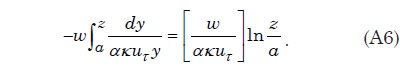
This states that for steady, uniform conditions the downward settling of sediment (–w c) balances the upward diffusion of sediment by turbulent eddies. Integrating once more with respect to height using y as the variable of integration yields

where a is a reference height near the bed where the concentration c(a) can be specified. In turbulent flow near the bed the eddy viscosity K_m for momentum is given by K_m = κu_τ z, where κ is the von Karman parameter, u_τ is the friction velocity, and z is height. Since the same eddies that diffuse momentum vertically also diffuse mass, one can represent the eddy diffusivity K_s as K_s = αku_τ z, where α is a constant of proportionality. For low sediment concentrations α≈ 1, and for high concentrations a value of 1.35 is commonly used. Substituting this expression for K_s into the right hand side of Eq. (A5) we find

Combining Eqs. (A5) and (A6) and using the fact that the Rouse parameter P = w/ku_τ, we obtain the following expression for the volume fraction c of sediment as a function of height z above the bed

This result is valid only near the base of the turbulent layer. To obtain a description that is applicable throughout the turbulent layer, it is necessary to use an eddy diffusivity that decreases more strongly with height. One such functional form commonly used yields an eddy diffusivity profile that is parabolic, decreasing to zero at the top of the turbulent layer at z = h and approaching αku_τz near the base of the layer. It is expressed as K_s = ακu_τ z(1–z/h). Substitution of this quadratic eddy diffusivity into Eq. (A7) yields what is known as the Rouse profile,

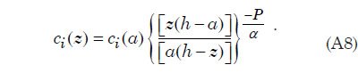
Since the Rouse parameter depends on particle settling velocity which in turn depends on particle size, we divide the sediment into a finite number of sediment classes according to particle size which we designate by the subscript i. Eq. (A8) then provides a separate vertical distribution of volume fraction for each sediment class.

Integrating Eq. (A8) with respect to height from a to h, noting that

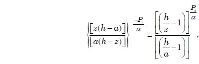
we obtain the following expression for the carrying capacity F_i of the flow for each sediment class

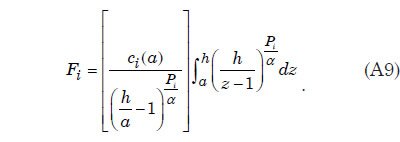
We choose the reference height a to be constant with a value of 1 cm (0.39 in). Since c_i(a), the sediment volume fraction at height a, is dimensionless, we note that F_i, has units of distance. F_i represents the total thickness of sediment of class i that the flow can suspend. For purposes of the computation, because, as explained below, we impose a severe limit on the sediment volume fraction at each height, we take c_i(a) to be unity. Note that F_i then depends only on the Rouse parameter P_i, of the sediment class and the depth of the turbulent layer h. For practical reasons, we divide the height coordinate z into a number of discrete zones or layers, indexed by k, and compute a sediment carrying capacity F_i^k for each layer. The total column carrying capacity F_i is then given by F_i = ΣF_i^k, where the summation is over k. In the illustrative cases we describe later, we use a total of seven vertical layers of fixed thickness to represent the sediment profile in the turbulent flow.

Turbulent water can maintain only a limited volume fraction of sediment in suspension. Based on the work of Bagnold (1966), the limiting volume fraction at any given height in the flow, over all sediment classes, is about 0.09. We impose this limit in each of the vertical layers at each lateral grid point in the computational mesh.

Appendix D: Settling Speed of Sediment Particles

As we have seen, the ability of a turbulent flow to suspend sediment particles and maintain them in suspension depends on the settling velocity w of the particles. The Rouse parameter P that occurs as the exponent in the vertical sediment distribution formula (A8) involves the ratio of the settling velocity w to the friction velocity u_τ of the turbulent flow. A great deal of experimental effort has been invested to characterize the settling velocity of sediment particles over the past 60 years. To obtain appropriate values for w we utilize a simple formula developed by Jiménez and Madsen (2003) that provides a good fit to the experimental measurements for grain sizes between 0.063 mm (0.0025 in) and 1 mm (0.039 in), covering the range from very fine to coarse sand. This formula is

with Y = [(s – 1) gd]_½ and S = 0.25 d Y/ν, where d is the nominal grain diameter, s is the specific gravity of the sediment grains, g is gravitational acceleration, ν is the kinematic viscosity of water, and A and B are constants arising from the fit to the data. We assume a specific gravity s for sand of 2.65, the value for g to be 9.8 m/s, and a kinematic viscosity ν for water of 10^-6 m²/s. The values for the constants A and B provided by Jiménez and Madsen (2003) are A = 0.954 and B = 5.12. For each sediment class i with mean nominal grain diameter d_i we apply (A10) to obtain the settling velocity w_i for that sediment class. For the case described in this paper we choose three sediment classes with nominal grain diameters d_i of 0.063 mm (0.0025 in), 0.25 mm (0.010 in), and 1 mm (0.039 in), corresponding to fine sand, medium sand, and coarse sand, respectively. Clay and silt is assumed to flocculate to form particles that display settling behavior identical to that of fine sand.

Appendix E: Erosion and Deposition

At present the erosion model is very simple. Since our interest is capturing the most salient aspects of the global Flood cataclysm in which water velocities reach several tens of meters per second, we neglect erosion processes at low water velocities and instead focus on cavitation-driven erosion which occurs at higher water velocities and results in extreme erosion rates. Cavitation involves the formation of water vapor and air bubbles which occurs when local fluid pressure drops below the vapor pressure of dissolved air (Arndt 1981). Cavitation damage arises when these bubbles are carried into regions of higher pressure and implode in the vicinity of the water-rock interface. The pressure spikes generated by the implosion and collapse of these bubbles are typically on the order of several hundred MPa, or several thousand atmospheres (Momber 2003). Such pressure pulses exceed the shear strength of most silicate minerals. They therefore damage and erode the lattices of individual crystals that comprise a polycrystalline rock (Momber 2003).

Whipple, Hancock, and Anderson (2000) provide the following simple expression to describe the rate ė_c of surface degradation in m/s from cavitation erosion

where E is a proportionality constant, u is the flow velocity just above the bed (assumed at height z = a), and u_cav is a cavitation threshold velocity. We adopt this simple relationship to represent cavitation in our model.

What values for q, u_cav, and E might be appropriate for representing the extreme conditions expected for a cataclysm on the scale of the Genesis Flood? Experimentally determined values for the exponent q as large as 7 have been reported (Murai et al. 1997). Falvey (1990) assumes a value for q of 6. Several authors put q in the range of 5–7. We choose a value for q of 6. Note that with q equal to 6, doubling the difference between u and u_cav increases the cavitation erosion rate by a factor of 64. The cavitation threshold velocity u_cav depends of the flow depth, fine sediment concentration, dissolved air content, and Reynolds number. Chanson (1997) observes that on chute spillways and bottom outlets, cavitation damage can begin to occur at clear water velocities of between 12 to 15 m/s. Falvey (1990) suggests that cavitation can begin to occur in spillways at velocities as low as 10 m/s. In our cavitation treatment we choose a value for u_cav of 15 m/s.

The multiplicative factor E in Eq. (A11) is not that well constrained by experimental data. Falvey (1990, 34) mentions an experiment in which a 13 mm (0.5 in) hole was produced in concrete over a period of 3 hours by a 30 m/s jet, but almost no details of the experiment are provided. These numbers suggest a cavitation erosion rate of 1.2 × 10^-6 m/s. More recently Momber (2003) reports experimental work to measure relative rates of cavitation erosion for various types of rocks and concrete using a cavitation chamber. Crucial details of the experiment are not included in the paper. Nevertheless, erosion rates provided in mg/s and the area of damage from the photographs in the paper imply erosion rates for granite and rhyolite on the order of 4 × 10^-5 m/s. In light of the measurements presently available, we view the value we have chosen (1 × 10^-5 m/s for a water speed of 20 m/s) as reasonable. The discovery that cavitation can be usefully applied to rock drilling is prompting laboratory studies pertaining to these applications (e.g., Momber 2003). This suggests that more experimental data for the cavitation regime of extremely high water velocities may soon be forthcoming.

It has also been proposed that cavitation may operate in conjunction with abrasion by suspended sediment particles to give erosion rates much greater than by either process alone. In attempting to account for many field examples of streambed erosion of massive, coarsely jointed rocks, especially features of fluting and pot-holing, Whipple, Hancock, and Anderson (2000), in the context of abrasion erosion by the suspended sediment load, remark:

Although one might argue that much of the suspended sediment flux passes through the system without much interaction with the channel boundaries, channel reaches where joint block plucking is inhibited typically develop significant and stable topographic irregularities, which generate intense vortices that bring the suspended load into contact with the bed. These vortices in fact focus abrasion damage on specific areas of the bed, resulting in the initial development of flutes and potholes. Once flutes and potholes begin to form, a strong positive feedback develops because the developing microtopography of the erosional form enhances and stabilizes the vortex structure, further strengthening the localized attack of abrasion by suspended particles. Finally, it is plausible that the inception of cavitation bubbles down the cores of vortices contributes to the focusing of erosion in flutes and potholes, as has been argued by some previous investigators (Baker 1974; Wohl 1992; O’Connor 1993). If cavitation indeed occurs in natural systems, the likely onset of cavitation within vortices during high-velocity flow may help explain the apparent dominance of fluting and potholing over abrasion wear by large, vigorously saltating particles. (Whipple, Hancock, and Anderson 2000, 8)

By the phrase, “vigorously saltating particles,” they are referring to bouncing bedload particles as opposed to particles suspended in the turbulent flow. They have already argued that the erosion rate from suspended sediment abrasion, apart from cavitation enhancement, ought to scale with the fifth power of the velocity just above the bed (Whipple, Hancock, and Anderson 2000, Eq. 10), and hence that it can possibly be comparable to the erosion rate they give for cavitation erosion. The two processes acting together must certainly involve rates much higher than either acting alone. Nevertheless, in our model we include only cavitation erosion and choose a value for u_cav of 15 m/s, a value for q of 6, and a value for E of 0.00001/(20–15)⁶ = 6.4 × 10^-10, which implies an erosion rate of 10^-5 m/s or 10 micrometer/s for a flow velocity at of 20 m/s at height z = a. We believe this to be very conservative for the velocity range in which cavitation occurs.

The deposition treatment is straightforward. Suspended sediment in the bottommost layer which is in excess of the carrying capacity of that layer is declared to be deposition. At each grid point the newly deposited sediment is added, by class, to a sediment deposition array and is also removed from the sediment suspension array for the bottommost vertical layer. This test is performed in the time stepping process after the new time level water column heights and velocities have been computed, after the suspended sediment profiles have been updated to account for the water transport, and after the new sediment carrying capacities have been computed. If the turbulent flow has not reached its capacity to suspend sediment and if the flow is sufficiently rapid to erode the base, we allow for erosion and suspension of the resulting eroded particles.

For our application, we account for the possible presence of a high concentration of sediment in the proximity of the surface. We do this by scaling E by the factor (1 – 10C), where C = Σc_i(a) is the sum over all sediment classes of their volume fractions within the height interval 0.01–1 m (layer 1), with this sum restricted by the sedimentation treatment to be no larger than 0.1. This restriction implies that when the total sediment volume fraction within the bottommost layer reaches 0.1, erosion ceases. In addition, we limit E such that it does not exceed 20% of the residual column carrying capacity, that is, 0.2 times the difference between the column carrying capacity and the total sediment load. For simplicity, we use these parameter values regardless of the flow depth and Reynolds number. When the bed material is sediment and not crystalline bedrock, we use the same parameters except that we increase E by a factor of three to account for the relative softness of the sediment. A test is made to ensure that all the existing sediment cover is eroded before any bedrock erosion occurs.

We assume further that cavitation degrades crystalline granitic bedrock into a distribution of particle sizes corresponding to 70% fine sand, 20% medium sand, and 10% coarse sand. This choice is motivated primarily by our assessment of the distribution that is characteristic of the earth’s sediment record. Implicit in this assumed distribution of particle sizes is the additional assumption that clay and silt-sized particles flocculate and behave as fine sand in their settling behavior. In addition, for purposes of this exploratory study, we ignore the carbonate sediments. We also note that experiments that provide a reliable particle size distribution from cavitation acting on crystalline silicate rocks are mostly lacking at this point in time.

After the erosion calculation has been performed, the newly eroded sediment is added to the suspended sediment profile by dividing the eroded sediment thickness, for each sediment class, by the height of the water column and multiplying by layer thickness for the contribution to each layer. Since it is possible in a given layer for the sediment concentration to exceed the carrying capacity, we address this situation. After the new time level water column heights and velocities have been computed, after the suspended sediment profiles have been updated to account for the water transport, and after the new sediment carrying capacities have been computed, but before the erosion calculation has been performed, we allow settling of sediment into the layer below. The amount transferred equals the time step (in seconds) multiplied by the settling rate (in meters per second) of the particular sediment class but limited by the excess of sediment in the layer (in meters) relative to the layer carrying capacity (in meters). We begin the procedure with the topmost layer.

The cumulative amounts of erosion and deposition, as well as the instantaneous amounts of suspended sediment by class, as a function of position over the surface, are tracked as the time stepping proceeds.

Appendix F: Effect of Sediment Load on Topography

It was found early in the testing the model that sediment thicknesses of several hundreds of meters routinely arise. When such large thicknesses were allowed to augment the original continent topography with no isostatic compensation whatsoever, a type of numerical instability was observed. This behavior involved the formation of localized mounds of sediment, typically a few hundred kilometers across and hundreds of meters high. This topography, in turn, forced the water flow to become concentrated in channels between these sediment mounds and for enhanced deposition to occur on top of the mounds where the flow depths and velocities were small. The higher the mounds grew, the stronger this tendency became. A simple remedy for this problem was to include some degree of isostatic compensation to allow the basement to subside in response to the sediment load above it. The compensation scheme chosen provides 10% compensation for loads less than 400 m (1312 ft), increasing to 30% compensation for a load of 1200 m (3936 ft) and 50% compensation for a load of 2000 m (6561 ft). For the portion of load in excess of 2000 m (6561 ft), 90% compensation is applied. Symmetrical compensation is implemented for the negative loads produced by material removed by bedrock erosion. Certainly, this prescription is only one of many that could have been chosen. Its main features include that the compensation is instantaneous, that the fraction of compensation increases monotonically with increasing sediment load height, and that there is almost complete compensation for loads greater than 2000 m (6561 ft) in thickness. The assumption that the compensation is instantaneous would, at first, seem difficult to justify, even as an approximation. However, when one takes into account the extreme reduction in rock strength throughout the mantle caused by the stress weakening mechanism associated with runaway lithospheric slabs and mantle plumes, it becomes more plausible. Calculations show that the weakening, which starts in the vicinity of a slab or plume that is entering the runaway regime, quickly spreads to encompass the entire mantle. The reduction in rock strength throughout the mantle then approaches a factor of a billion. This reduction in rock strength also affects the lithosphere. It implies a rapid response of the continental lithosphere to surface loading during the Flood while the mantle is in its weakened state.

Such nearly instantaneous compensation was found to suppress the unexpected behavior in an effective manner. However, the behavior may well not be computational but rather may actually be reflecting physical reality. As such, it clearly merits further study. This is especially so given that the tendency of the flow to form mounds of sediment yields more vigorous localized water flow, more intense erosion, and ultimately greater volumes of sediment. However, such further exploration will be deferred until later and is considered beyond the scope of this present paper.

Appendix G: Solving for the Water Flow Using the Shallow Water Approximation

To describe the water flow over the earth we utilize the so-called shallow water equations applied to a rotating sphere. By shallow water it is understood that the water depth is everywhere small compared to the horizontal scales of interest. The ocean basins today have mean depths of about 4 km (2.5 mi) while the computation grid for the earth’s surface for the cases we describe in this paper has a horizontal grid point spacing of about 120 km (74.5 mi). The expected water depths over the continental regions where our main interest lies are yet much smaller than those in the ocean basins. The shallow water approximation is therefore an appropriate one for this problem, one that allows the water flow over the surface of the globe to be treated in terms of a single layer of water with laterally varying thickness. What otherwise would be an expensive three-dimensional problem now becomes a much more tractable two-dimensional one.

The shallow water equations on a rotating sphere may be expressed (Williamson et al. 1992, 213)

and

where h is water depth, u is horizontal velocity (on the sphere), f is the Coriolis parameter (equal to 2Ω sin θ for rotation rate Ω and latitude θ), k is the outward radial unit vector, g is gravitational acceleration, and h^† is the height of the free surface above some spherical reference surface. Here it is assumed that the water is homogeneous in composition, incompressible, and inviscid. If h_t denotes topography on the sphere, then h^† = h + h_t. The d/dt operator is the material or substantial or co-moving time rate of change of an individual parcel of fluid. The ∇ operator is the spherical horizontal gradient operator and the ∇• operator is the spherical horizontal divergence operator. Symbols in bold font correspond to vector quantities. Eq. (A12) is an expression of the conservation of mass, while Eq. (A13) is an expression of the conservation of linear momentum. As mentioned above, this two-dimensional formulation in terms of a single layer in the radial direction is appropriate when the water depth is small in comparison to the important horizontal length scales.

In our problem the water depths above the continental regions are much smaller compared to those in the oceanic regions, and in these continental regions where the water is shallow we expect strong turbulence. Therefore, the assumption that the flow is inviscid is not an appropriate one, and we need to account for the strong drag that occurs at the continent-water interface. A simple means for doing this is to add a bottom friction term on the right hand side of Eq. (A13) of the form –βu/(h + 1), where β is a scaling parameter with units of m/s. Because the terms in Eq. (A13) have dimensions of force per unit mass, this drag term requires the division by water depth h to be consistent. The addition of 1 to h in the denominator is to prevent the overall term from becoming excessively large as the water depth approaches zero. It is also common in ocean models to include in the momentum equation a so-called eddy viscosity term that seeks to represent the effects of turbulence on scales not resolved by the computational grid. The simplest such formulation is a term proportional to the 2-D Laplacian operator ∇² = ∇•∇ on the sphere applied to the velocity field, that is, a term of the form γ∇²u, where γ is a scaling parameter with units m2/s. Note that γ depends on the grid resolution. Typical values are 1 × 10^-3 for β and 2 × 10^-11 for γ when the grid spacing is 120 km (74.5 mi). Adding these two terms to the right hand side of the momentum Eq. (A13) yields

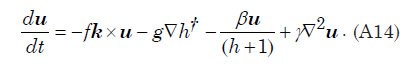
Note that in continental regions the water depth can decrease to zero. We therefore constrain the water depth h always to be non-negative and the water velocity u to be zero when h is zero. We also constrain the right-hand side of Eq. (A14) to be zero when h is zero.

Eqs. (A12) and (A14) are solved in discrete fashion on a mesh constructed from the regular icosahedron as shown in Fig. 1. A separate spherical coordinate system is defined at each node such that the equator of the system passes through the node and the local longitude and latitude axes are aligned with the global east and north directions. This approach has the advantage that the coordinates are almost Cartesian and only two (tangential) velocity components are needed. A semi-Lagrangian formulation (Staniforth and Cote 1991) of Eqs. (A12) and (A14) is used which involves computing the trajectories during the time step that end at each node. Values for h and u at the beginning of the time step at the starting point of each trajectory are found by interpolating from the known nodal values at the beginning of the time step. Changes in h and u along the trajectory are computed using Eqs. (A12) and (A14). This Lagrangian-like method eliminates most of the numerical diffusional noise that is associated with Eulerian schemes. A second-order accurate interpolation scheme is used to find the starting point values of the trajectories. This formulation using the icosahedral mesh has been carefully validated using the suite of test problems developed by Williamson et al. (1992). It also forms the basis for the global weather forecast model known as GME developed in the late 1990s by the German Weather Service which in now used by more than 20 other nations (Majewski et al. 2002).