
Research conducted by Answers in Genesis staff scientists or sponsored by Answers in Genesis is funded solely by supporters’ donations.
Abstract
For more than two decades, recent creationists have used the supposed lack of old supernova remnants, and particularly the lack of stage three supernova remnants, as an argument for recent origin. However, reexamination of the data shows that there indeed are old supernova remnants, and that stage three supernova remnants have been identified. Therefore, this may not be a good argument for recent origin, and I discourage recent creationists from using it.
Keywords: supernovae, supernova remnants
Introduction
For more than two decades, supernova remnants (SNRs) have been used by creationists as evidence for recent origin (Davies 1994, 2006, 2007). A supernova is a powerful explosion of a star. Depending on several factors, the core of the star that explodes typically is transformed into a compact object, either a black hole or a neutron star. However, the nature of type Ia supernovae is very different, and no remnant may be left behind. For a discussion of supernovae and stellar remnants in the creationary literature, see Faulkner (2007). A supernova explosion disperses the matter in the envelope (the region of a star exterior to its core) of the progenitor star. The initial rate of expansion of the material ejected by a supernova typically is thousands of km/s. As this matter expands into space, it develops into a structure that we recognize as a SNR. Astrophysicists modeling the evolution1 of SNRs recognize three stages. The first two stages are relatively short, while the third stage lasts much longer. Some sources consider dispersal, and hence disappearance, of a SNR as a fourth stage, though this delineation is uncommon, and it would be very difficult, if not impossible, to observe SNRs in this stage. The essence of the argument for recent origin is that astronomers observe SNRs in the first two stages, but not in the third stage. Astronomers use models to interpret their observations to estimate ages of SNRs. The recent creation claim is that the oldest SNRs are only thousands of years old, while theory would dictate that if the universe is billions of years old, we ought to see many SNRs much older than this, particularly in stage three (the stages will be explained later).
Understandably, critics of recent creation have responded (Moore 2003; Plait 2002, 198–200; Ross 2008). Moore’s evaluation is the most complete, alleging several problems with the SNR argument for recent origin, ranging from use of outdated references and misquoting or quoting out of context to overlooking the evidence of examples of stage three SNR that are very old. To date, only one short critical evaluation from within the recent creation community has appeared (Setterfield 2007). Hence there is a need for a more comprehensive critical evaluation of this question in the creation literature. Here I primarily will consider the claims that we do not see stage three SNRs and that the estimated SNR ages are consistent with recent origin but not consistent with a universe that is billions of years old.
Theoretical Understanding of SNRs
Draine (2011, 429–439) has a good summary of the three stages of SNRs. Stage one is the free-expansion phase. This means that the expanding material encounters little resistance, because the density of the ejected material greatly exceeds the density of the surrounding interstellar medium (ISM). Normally, an expanding gas cools due to work accomplished by the gas, but since in stage one the gas is virtually freely expanding, little work is done, so the temperature of the gas is nearly constant. Nor is the velocity of expansion slowed much in stage one. The velocity of the expanding ejecta is far higher than the sound speed in the surrounding material, so the ejecta drives a fast shock through the ISM. The supernova remnant is the matter contained within this shock front. As the expansion continues, the density of the expanding ejecta drops, so eventually the pressure in the shocked ISM exceeds the gas pressure of the ejecta. This condition allows a reverse shock to propagate toward the center of the SNR. To distinguish the reverse shock from the outgoing shock, the outgoing shock is called the blastwave. The reverse shock slows the material within the SNR and heats it to very high temperature. The reverse shock becomes important when the blastwave has swept up mass that is comparable to the mass of the ejected material. The timescale for this and the timescale for complete penetration of the SNR by the reverse shock are approximately the same. Obviously, these timescales depend upon several quantities, such as the amount of ejected material, the ejected material’s speed, and the density of the ISM encountered by the expanding SNR. Estimates for these timescales varies from decades to centuries. For instance, the SNR Cassiopeia A (Cas A)2 is estimated to be a little more than three centuries old, and it still is in the free expansion stage. This is a very old stage one SNR.
The second stage is the Sedov-Taylor (alternately, Sedov, or adiabatic) phase. The reverse shock heats the gas in the SNR to exceedingly high temperatures. Much of the matter becomes concentrated in an expanding shell behind the blastwave. The greater density in the shell facilitates the radiation of heat, eventually cooling the shell below the temperature of the wavefront. Sedov worked out a relationship between the radius of the shock front, r, the energy released by the supernova, E, the number density of hydrogen atoms in the ISM, n, and the age of the supernova, t (Minkowski 1968, 632):
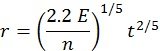
Depending on the units used, this equation will have different constants, but the functional dependence of the four variables remains. The energy released in a supernova is on the order of 1051 ergs. Astronomers believe they have a good understanding of the number density of hydrogen atoms in the ISM. The angular diameter of a SNR is relatively easy to measure, so if the distance to a SNR can be determined, the linear size can be computed. The remaining variable is the age of the SNR. Therefore, the Sedov relation often is used to estimate the ages of SNRs in the second stage. Theorists expect that the second stage typically lasts tens of thousands of years.
The radiative phase brings the second stage to a close and ushers in the third stage. With the shell of matter behind the wavefront significantly cooler than the matter on the wavefront, pressure rapidly drops, and the blastwave briefly stalls. However, the very low density, but very high temperature, gas in the interior drives the expansion outward. This is the third stage, or snowplow phase, so called, because the wavefront continues to sweep up material ahead of it. Despite its exceedingly high temperature, the interior of the SNR has such low density that it cannot cool easily. Much of the cooling is achieved by emission from ionized metals in the gas. We can detect this emission, so this stage sometimes is called the radiative phase. Through all this, the expansion rate of the wavefront continually slows. The original expansion speed was many thousands of km/s, but eventually the expansion velocity slows to less than 100 km/s. When the speed of advancement reaches the sound speed in the ISM, the shock wave rapidly transitions into a sound wave, after which, the SNR fades into the ISM. The timescale for this may be on the order of a million years.
This is the theoretical understanding of supernova remnants, but the real situation is much more complicated. First, keep in mind that there is some overlap between the three stages, so it may be difficult to assign a unique stage to a SNR. Second, the model assumes a uniform, very cool, very low density ISM. While the ISM has very low density compared to any terrestrial standards, it is anything but uniform. Density in the ISM can vary by several orders of magnitude. Because of its low density, many different temperatures can coexist in the ISM. These temperatures range from only a few K to a million K. As an expanding SNR encounters different conditions in the ISM, different portions of its periphery interact differently. A third complication is that models generally assume a symmetrical explosion, but observations reveal that some SNs are asymmetrical. For instance, images of the best-studied SNR, the Crab Nebula (Fig. 1), is noticeably elliptical, indicating that the expansion is slightly greater in one direction than in the other direction. But the images reveal only two dimensions, both in the plane of the sky. The motion in our line of sight (perpendicular to the plane of the sky) is measured spectroscopically via the Doppler effect. This velocity likely is different from the other two directions. However, images of most SNRs are nearly circular, and those that are not circular have only slightly elliptical shapes, indicating that expansion of SNRs typically varies far less than a factor of two in different directions. A fourth complication is the natal kicks sometimes given to neutron stars produced by SN explosions. This is evidenced by the high velocity (hundreds of km/s) many neutron stars have relative to their associated SNRs. Some pulsars are moving so rapidly, they lie outside their SNRs. We call these pulsars runaway pulsars. Runaway pulsars indicate some asymmetry in SN explosions.
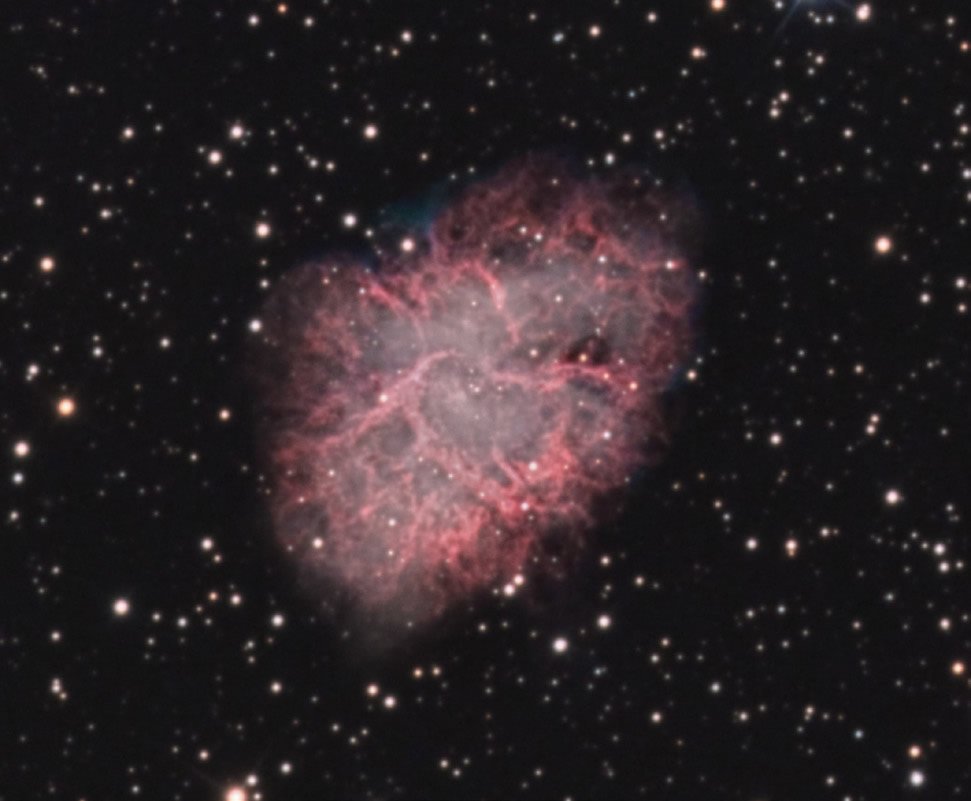
Fig. 1. The Crab Nebula. (Photograph: Glen and Katrina Fountain).
A fifth complication is that observational criteria differ greatly from the theoretical history. Left unaddressed in the simple model of three stages above is the effects of a neutron star, if any, left behind by the supernova explosion that birthed the supernova remnant. We usually detect neutron stars as pulsars. Pulsars manifest themselves by their rapid rotation and strong magnetic fields. These two factors combine to interact complexly with charged particles to produce two beams of radiation. These beams are aligned with the magnetic poles of the neutron star. The theory is that the resulting “light curve” of the pulsar results since the magnetic poles and rotation axes generally do not coincide, so as the neutron star rotates, the radiation beams sweep out a cone, similar to that swept out by a searchlight. If the earth lies near the cone, we detect periodic flashes, or pulses, as one of the beams rotates (hence, the name “pulsar”). Another complex interaction between winds generated by the neutron star and its powerful, fast-moving magnetic field produce a type of nebula called a plerion or pulsar wind nebula. A plerion is contained within the supernova remnant. The best-known supernova remnant, the Crab Nebula (see Fig. 1), contains a plerion around its central pulsar, the Crab Pulsar (PSR B0531+21)3. A plerion is much smaller than the SNR.
SNRs do not instantly go from one stage to the next stage. Rather, there is some overlap and time for transition. Furthermore, the different stages are not that obvious in observations. Instead, observations of a SNR must be interpreted in terms of models to determine what stage it might be in. Observationally, there are three types of SNRs:
- Shell-like
- Composite
- Mixed morphology
As the name implies, most of the radiation from a shell-like SNR comes from a shell. They usually appear as a ring of material. There is no plerion within the shell, probably because the supernova that created the SNR did not produce a neutron star. The best example of a shell-like SNR is Cassiopeia A. A composite SNR has a shell, along with a plerion within the shell. The best example of a composite SNR is the Crab Nebula. A mixed morphology SNR has a radio shell with interior X-ray emission. A few SNRs are both composite and mixed morphology SNRs.
Finally, a sixth complication is the limits of detectability of SNRs. SNRs typically are located near the galactic plane. There is much dust and gas concentrated in the galactic plane. The dust and gas obscures radiation from distant objects near the galactic plane. This is particularly a problem in the optical part of the spectrum, but is far less of a problem in the radio, where many SNR observations are made. There is more penetration through the dust and gas of X-rays and other highly energetic radiation than in the optical. Light intensity decreases with the inverse square of the distance, so detection and observation of distant SNRs is problematic as well. As Davies (1994) briefly discussed, these observational limitations make it impossible to detect most galactic SNRs. Therefore, the SNRs that we observe are but a fraction of the total SNRs in the galaxy. It is not clear what fraction of total galactic SNRs we detect. There are other selection effects at work. See Green (1991) for a good discussion of the selection effects in observing galactic SNRs.
Empirically, there is a relationship between the surface brightness of SNRs measured at radio frequencies (Σ) and their sizes (d or diameters). This is expected, because SNRs ought to fade as they age, and as they age, they expand, so their diameters increase. This relationship normally is expressed as the Σ–d relation. Once calibrated, the Σ–d relation is very helpful in establishing physical characteristics of SNRs. This relation primarily works for shell-like SNRs, but it can be applied to composite SNRs under certain conditions. Application of the Σ–d relation to the observed surface brightness of a SNR remnant allows computation of the SNR’s size. Knowing the linear size and the measured angular size of a SNR, computation of the distance quickly follows. The combination of other observational data with the size and distance allows calculation of other physical properties, such as age.
This approach is decidedly different from that of Davies (1994), who relied upon a plot bounded by limitations of observation. Davies’ Figures 1 and 2 were plots of the diameters of SNRs, D, as a function of distance, d. Diameters were expressed in pc (parsecs),4 while distances were expressed in kpc (kiloparsecs). The intersection of three curves define a roughly triangular region of the plot where SNRs were expected to be observable. One curve is a limitation on maximum size, while one curve was a limitation of minimum size. Most important was the third curve limiting the minimum flux of visible SNRs. Davies’ Figure 1 contained no data, but merely showed the region of the plot where SNR were expected be observable. Figure 2 was a reproduction of Figure 1 with points representing measured sizes and distances of SNRs. While there was a clump of points representing smaller SNRs, there was a noticeable lack of larger (older) SNRs. Note that there was no comparison of explicit age measurements, but rather an inferred lack of old SNRs based upon a lack of large SNRs. That is, there were no explicit SNR ages presented. Also keep in mind that Davies’ two figures were based upon a particular model of SNR evolution from the literature. If SNRs evolve differently from the model, the conclusions based upon the model may not be correct.
Rather than replicate Davies’ indirect method based on a single model, I will present measurements of SNR ages from the astronomy literature, each based upon data taken for SNRs interpreted with a variety of models. As I shall show, there are many examples of old SNRs.
An Important Case Study: The Crab Nebula
It is best to begin discussion of the very young, but the best studied SNR, the Crab Nebula (see Fig. 1). For a discussion of the Crab Nebula in the creationary literature, see DeYoung (2006). While normally referred to as the Crab Nebula, there are other, less commonly used, names. The most common alternate name is M1.5 The Crab Nebula has been a remarkable laboratory for studying SNRs. An important aspect is the Crab Nebula contains one of the first pulsars discovered, PSR B0531+21, or, as it is more commonly known, the Crab Pulsar.
Another important aspect is that we know the exact age of the Crab Nebula and its pulsar. This allows us to test some of our methods for determining the ages of SNRs. From historical records, we know that a supernova appeared in the constellation Taurus in July AD 1054. The supernova faded to invisibility over the next two years. In 1731, more than a century after the invention of the telescope, John Bevis was the first to spot a nebula at the location of the supernova. In 1840, William Parsons, third Earl of Rosse, saw filaments in the nebula, which reminded him of the appearance of a crab, from which the nebula’s common name arose. However, it was not until the early twentieth century that astronomers came to realize the significance of the coincidence of the location of the AD 1054 supernova and the Crab Nebula. Also in the early twentieth century, astronomers comparing photographs of the Crab Nebula taken a few years apart saw that it was noticeably expanding.
Observed expansion of the Crab Nebula is useful in measuring its age, distance, and size. The change in positions of filaments near the perimeter of the Crab Nebula measured on two photographs divided by the time between the photographs yields the proper motions of the filaments. Proper motion, µ, usually is expressed in units of arcseconds per year (″/yr). Division of the angular distance of a knot of material from the center of the Crab Nebula by its proper motion reveals the time since the expansion began, and hence the age of the SNR. Normally, the ages determined from numerous knots are averaged. The date of the origin of the Crab Nebula using this method is AD 1140 (Trimble 1968). This date is 90 years after the recorded date of the SN, producing an age that is about 10% younger than the known age of the Crab Nebula. This is explained by acceleration of the expansion of the SNR powered by the pulsar near its center (Bejger and Haensel 2003).
Space motion, the velocity of an object in space, can be divided into two components, the radial velocity, VR, along our line of sight, and the tangential velocity, VT, perpendicular to our line of sight. Both are expressed in units of km/s. The distance, D, is measured in pc. Proper motion, tangential velocity, and distance are related by:
We do not know the tangential velocities of material in the Crab Nebula, but we can measure the radial velocities spectroscopically. If we assume a spherically symmetric expansion, then we can equate the tangential and radial velocities, and the distance to the Crab Nebula follows. Trimble (1973) has an excellent discussion of the history of this method of finding the distance to the Crab Nebula. She found the distance to be 1930 pc (6300 light years). From the elliptical shape of the Crab Nebula, we know that the expansion is not symmetrical. However, the known asymmetry in the two-dimensional images suggests that the uncertainty introduced by the assumption of symmetry is far less than a factor of two. Knowing the distance, we can use the angular size of the Crab Nebula measured on photographs to estimate its size (its longest axis is a little more than 10 light years across).
Pulsar periods are extremely regular. However, pulsars gradually slow their rotation as their considerable rotational kinetic energy is tapped to power the radiation they emit. The rate of change in a pulsar’s period can be used to estimate the pulsar’s spin-down age or characteristic age, τ. Let P be a pulsar’s period and Ṗ be the time rate of change (derivative) of the period. A simple expression for the characteristic age is

For instance, the characteristic age of the Crab Pulsar using this formula is 1240 years (Haensel, Potekhin, and Yakovlev 2007, 37). This is 30% longer than the known age of the Crab Pulsar. Why the discrepancy? There are several factors. The above relationship is a simple form—more accurate formulations exist. The observations are subject to noise. From time to time, pulsars exhibit glitches, slight discontinuous changes in their periods. Astronomers believe that glitches result from readjustment of pulsars as their period of rotation decreases. Rapidly rotating neutron stars are distorted into oblate spheroids. As the period of rotation decreases, the equatorial radius of the oblate spheroid decreases. However, the matter in neutron stars is very stiff, so their matter does not readjust continuously, but rather in drastic steps. Finally, millisecond pulsars have been spun-up via interactions with a close binary companions. This interaction interferes with the manner that neutron stars normally would evolve, so characteristic ages of millisecond pulsars are meaningless. With these caveats, it is encouraging that the Crab Pulsar characteristic age is so close to its true age. It is likely that when appropriately used, the characteristic ages of pulsars are well within a factor of two of their true ages.
As an aside, the Crab Pulsar permits astronomers to probe the ISM. The presence of free electrons in the ISM subtly changes the speed of light. This effect, called dispersion, causes pulses observed at lower frequencies to arrive later than pulses observed at higher frequencies (Draine 2011, 102–105). From dispersion studies of Crab Pulsar pulses, astronomers have measured the column density of free electrons in the 6000-light year length line-of-sight between us and the Crab Pulsar. If we assume there is an effective average volume density of free electrons, division of the measured column density by the distance yields that average volume density. Assuming the average volume density of free electrons determined along the line of sight of the Crab Nebula is typical, astronomers can use dispersion measurements to measure the distance to any pulsar. In practice, kinematic studies of pulsars (briefly described below) can give us estimates of their distances, offering a check on electron volume density in the galaxy and this method of finding pulsar distances.
With the techniques developed and tested with the Crab Nebula and its pulsar, we can apply these techniques to other SNRs and any associated pulsars. Astronomers sometimes can measure expansion rates of SNRs, allowing direct measurement of SNR ages. When this is not possible, another method often is applied. We have a good understanding of the structure of the Milky Way galaxy, including the motions of objects as they orbit the galaxy. The average radial velocity of a SNR remnant can be interpreted to give a distance based upon a model of galactic kinematics. Most SNRs have low galactic latitudes, making this a simple calculation. The product of the angular size (in radian measure) and this kinematic distance yields the SNR diameter. Assuming a typical expansion rate, one can estimate a SNR’s age. Another way of doing this it to estimate limitations on detectability. This is the essence of Figures 1 and 2 of Davies (1994). Many papers on SNRs today use very developed models of SNRs to determine from observations the energy and luminosity of SNRs, which in turn yields their sizes. One can infer ages from these considerations as well. Finally, in some cases, SNRs have associated pulsars from which spin-down ages can be determined. When no estimate of a SNR’s age is directly possible, this establishes the age of the SNR. When astronomers can estimate a SNR’s age, the characteristic age of its associated pulsar acts as a check on direct age determinations of the SNR. Keep in mind that most SNRs do not have an associated pulsar.
Another Case Study: The Cygnus Loop
More recently, Davies (2006) discussed the Cygnus Loop.6 Spanning nearly 3°, the Cygnus Loop is one of the largest-appearing SNRs. In his catalogue of 294 SNRs, Green (2014) listed only two other SNRs that appeared slightly larger. This means that either the Cygnus Loop is among the larger SNRs, is among the nearer SNRs, or a combination of both. Distance estimates, and hence estimated ages, of the Cygnus Loop have varied, but recently there has been a decrease in both. The first age estimate was that of Edwin Hubble, who found an age of 150,000 years. According to Adams and Seares (1937, 189), Hubble measured the relative proper motions of NGC 6960 and NGC 69927 on photographs taken 27 years apart. These two nebulae are two of the brighter segments of the Cygnus loop, and are diametrically opposite, about 2½° from one another. Hubble found the two nebulae were separating at a rate of 0.06 arcseconds per year.8 This was an improvement upon an earlier measurement by Hubble of 0.1 arcsecond per year based upon photographs taken only 15 years apart (Hale, Adams, and Seares 1926, 118).9 The age of 150,000 years comes directly from dividing the separation of the two nebulae (2½° = 9000 arcseconds) by the rate of separation. However, the report included the qualifier “if the expansion has been uniform.” Undoubtedly, Hubble and others at the time understood the expansion of the loop probably had slowed, and so Hubble’s computed age merely was an upper limit for the age. Indeed, Minkowski (1958) made the first radial velocity measurements of Cygnus Loop, and he found an expansion velocity of 116 km/s. This is more than an order of magnitude lower than the initial speed of material ejected from supernovae. Previously, Zwicky (1940) and Oort (1946) were the first to suggest that the Cygnus Loop was a SNR, and that the speed of expansion had slowed tremendously due to collisions of the expanding gas with gas in ISM.
As previously discussed with the Crab Nebula, the distance, diameter, and age of SNRs are intimately related. Zwicky estimated the angular diameter of the Cygnus Loop to be 4.7° (approximately 50% larger than it actually is), and its linear diameter as 10 light years (about 3 pc). Zwicky did not explain the reason for assuming this linear diameter. This information corresponds to a distance of 39 pc, much closer than thought today. Using this data, along with assumptions about the initial speed of the ejected material and the density of the ISM, Zwicky computed the age of the Cygnus Loop at a little more than 10,000 years. Given how incorrect some of his assumptions were, the concordance of this age with the modern determination is remarkable. Minkowski (1958) used his measured expansion velocity to determine the distance of the Cygnus Loop to be 770 pc, and its diameter as 40 pc. However, the observed expansion, both in terms of radial velocity and proper motion, almost certainly had slowed via interaction with the ISM. Therefore, both Minkowski’s distance and size were too large. Despite this well-known caveat about slowed expansion, Minkowski’s distance and size estimates were widely accepted for years. Based upon this size and distance, Minkowski (1968, 657–658) used the Sedov model to compute the age of the Cygnus Loop as 67,000 years. Interestingly, in his earlier paper, Minkowski (1958) obtained the same age by simpler means. While this was about half Hubble’s age estimate, given the likelihood that the Cygnus Loop is much smaller than assumed, this age estimate probably was too high as well.
In a novel approach, Ilovaisky and Lequeux (1972a) obtained a luminosity function (Σ–d) for galactic SNRs. In a subsequent study, Ilovaisky and Lequeux (1972b) used their luminosity function to infer a galactic supernova rate. Since we cannot directly observe the galactic supernova rate due to interstellar extinction by dust, their goal was to derive an empirical galactic supernova rate by other means. They compared the observed supernova rates of other galaxies similar to our Galaxy (2–4 per century) in hopes of finding concordance. They generally found concordance, except for the Cygnus Loop, what they called “an interesting case.” The inferred supernova rate using the Cygnus Loop was approximately 315 years between supernova events, a Galaxy supernova rate (1/3 per century) an order of magnitude too low. To resolve this dilemma, they proposed that the published ages of the Cygnus Loop were too old. They suggested “the observed expansion velocity of the filaments, from which the age is derived, was significantly smaller than the velocity of the shock front.” To get a good fit to the assumed galactic supernova rate required quadrupling the shock front speed over the filament speed. This resulted in an age estimate of about 14,000 years, about one-tenth Hubble’s initial estimate. They based their work upon a great distance (they chose 800 pc) of the Cygnus Loop, using the “established” distance of 770 pc. Had they assumed a much smaller distance, they may have produced concordance with the standard supernova rate without decoupling the shock speeds and filament speeds so greatly. Ku et al. (1984) modeled X-ray data to determine an age of 18,000 years for the Cygnus Loop, while Miyata et al. (1994) also used X-ray data to determine an age of 20,000 years. Both studies concluded that the Cygnus Loop was near the end of the Sedov stage, soon to emerge into stage three. And as with previous studies, they assumed the distance was 770 pc.
Amazingly, in all these years, apparently no one questioned this distance and size of the Cygnus Loop, even though there was good reason to believe that they were too great. As mentioned before, recognition that the rate of expansion had greatly decreased would result in a smaller size and hence distance. However, there is another reason to believe the Cygnus Loop is much closer than had been thought. The Cygnus Loop has a relatively high galactic latitude (−8.5°). SNRs are strongly concentrated along the galactic plane, with many of them within 1° of the galactic plane. This is interpreted to mean the progenitor stars of supernovae lie close to the galactic plane. Additionally, any appreciable vertical distance from the galactic plane will result in low galactic latitude, if the object is far away. In Green’s catalogue of 294 SNRs (Green 2014), only four sources have galactic latitude greater than the Cygnus Loop. Unless the Cygnus Loop is exceptionally far from the galactic plane, it must be very close to have such a high galactic latitude.
Though it was not the main thrust of their paper, Braun and Strom (1986) reevaluated Minkowski’s spectral data, and, using Hubble’s proper motion, determined the distance of the Cygnus Loop to be 460 pc, about 60% what had been thought. This new distance did not attract much attention, but that of Blair et al. (1999) did. This team used the Hubble Space Telescope to remeasure the proper motion of filaments in the Cygnus Loop. Their result, 0.082 arcseconds per year, is 175% greater than Hubble’s original measurement. Furthermore, they combined this new proper motion with improved radial velocity measurements to conclude the Cygnus Loop was 440 pc away, in good agreement with Braun and Strom. Blair et al. (2004) confirmed this distance by showing that the spectrum of the star KPD 2055+3111.10 This star lies in the direction of the Veil Nebula (part of the Cygnus Loop), has absorption lines that only could be from the SNR. This places the star behind the Cygnus Loop, but constraints on the star’s properties indicate that the star is 600 pc away. This would be impossible if the Cygnus Loop were farther away than 600 pc. Blair et al. (1999) pointed out that reducing the distance to the Cygnus Loop alters other inferred properties as well. For our concern here, the 18,000-year age determination of Ku et al. (1984) reduces to 5000 years. Furthermore, this probably changes the status of the Cygnus Loop from very late Sedov-stage SNR to a moderate age Sedov-stage SNR.
In his paper, Davies (1994) recognized the role of the incorrect distance in inflating the age of the Cygnus Loop, but he also blamed an assumption of a number density of the ISM that was too large. He referenced Ilovaisky and Lequeux (1972b) as pointing out that the number density near the Cygnus Loop was closer to 0.1 than to 1.0, for he wrote:
It was this error in the density (of a factor of 10) that was partly the culprit for the age of the Cygnus Loop being so grossly overestimated in prior publications.
Examining the Sedov equation, one sees that the age is directly proportional to the square root of the number density. Therefore, a reduction of ten in the number density would result in a decrease in age by a factor of about three. However, Davies apparently misunderstood what Ilovaisky and Lequeux wrote. The low density (n ≈ 0.1) in the vicinity of the Cygnus Loop had been assumed for some time (Sholomitskii 1963). The justification for the low number density was a consequence of its relatively high galactic latitude corresponding to a relatively large distance from the galactic plane (Ilovaisky and Lequeux 1972b; Minkowski 1968). The density of the ISM is greatest on the galactic plane and decreases with increasing distance from the galactic plane. Hence, Ilovaisky and Lequeux were not surprisingly or reluctantly led to the lower density, but rightfully adopted it because of compelling reasons, as had others. Furthermore, a reduction in the distance to the Cygnus Loop results in a smaller distance from the galactic plane, which in turn increases the presumed number density. Hence, due to its relatively high galactic latitude, a decrease in distance to the Cygnus Loop tends to produce a younger computed age, but the corresponding increased number density in the ISM tends to increase this computed age. Davies missed this point, as he used the reduced diameter but an unrealistically low number density to obtain an age of 2400 years.
The thrust of Davies’ paper on the Cygnus Loop was to argue that perhaps other SNR ages similarly had been overestimated. However, the Cygnus Loop appears to be a unique situation. Furthermore, Davies concentrated on a supposed error involving the number density of the ISM, but that was a misunderstanding of the situation. At one time, the great age of the Cygnus Loop was problematic for recent creation (less than 7000 years old being Davies’ criterion). However, the latest age estimates of the Cygnus Loop are near or within the age limit of recent creation models, so it no longer is a problem. Davies’ other work on SNRs concerned the lack of old SNRs as evidence of recent origin. But if one can find examples of SNRs that are much older, and possibly SNRs that are in stage three, then it would call into question Davies’ work.
Measurements of Ages of other SNRs
Using variations on the techniques briefly described above, astronomers can measure the ages of other SNRs. What have these studies concluded? I briefly will survey the results of 17 selected SNRs.
Another loop structure identified as a SNR is the Monoceros Loop (SNR G205.5+0.5).11 Wallerstein and Jacobsen (1976) determined that the Monoceros Loop is 150,000 years old. Graham et al. (1982) applied the surface brightness–distance relationship of Caswell and Lerche (1979) to their radio observations to conclude that the Monoceros Loop is 1600 pc away and has a diameter of 115 pc. Their derived age was 150,000 years agrees with that of Wallerstein and Jacobsen (1976). In their discussion, Aharonian et al. (2004) identified the Monoceros Loop as being in the Sedov phase (stage two) and gave its age as 30,000–150,000 years. This range of ages apparently came from the literature, but without reference (I was not able to find such young age estimates for the Monoceros Loop in the literature, so 30,000 years may be merely a rough estimate). Similarly, Dirks and Meyer (2016) described the Monoceros Loop in their introduction as “a well-evolved SNR” with an age of approximately 100,000 years.
As the name implies, the Lupus Loop (SNR G330.0 + 15.0) is a circular emission feature in the constellation Lupus. However, unlike the Cygnus and Monoceros Loops, the Lupus Loop is not visible optically, but rather has been detected in the radio and X-ray parts of the spectrum. It is coincidentally located near SN 1006 (SNR G327.6 + 14.6), a younger SNR from an unrelated supernova observed in AD 1066. The Lupus Loop has the distinction of having the highest galactic latitude (15°) of any object in the SNR catalogue of Green (2014) (SN 1066 has the second highest galactic latitude). Its high galactic latitude and its rather large angular size (the angular size is uncertain, but it is several degrees) suggest that the Lupus Loop is not far away, yet estimates of the distance vary. Leahy, Nousek, and Hamilton (1991) modeled X-ray observations to find a distance of 1200 pc and an age of 49,000 years. If this distance is correct, then the diameter of the Lupus Loop is between 50 and 100 pc.
There are several examples of agreement between ages of SNRs and the characteristic ages of their associated pulsars. For example, Harrus, et al. (1997) used a radiative-phase shock (stage three) model to determine an age of approximately 20,000 years for W44 (SNR G034.6-00.5),12 the same as the estimated age of its associated pulsar, PSR 1853+01. The concordance of these two ages determined from very different methods, one for the SNR and one for the pulsar, is a powerful argument that these ages are reasonably correct. Similarly, Matthews, Wallace, and Taylor (1998) termed SNR G055.0+00.3 “a highly evolved supernova remnant,” with an estimated age of approximately 1,000,000 years, matching the 1.1 × 10⁶ years characteristic age of PSR J1932+2020, the pulsar thought to be associated with SNR G055.0+00.3. Another example is CTB 80 (SNR G068.8+02.6).13
Safi-Harb, Ögelman, and Finley (1995) noted that the estimated age of the HI shell of CTB 80 and the spin-down age of its associated pulsar, PSR 1951+32, agree well (within 15%), and indicate an age of approximately 105 years. More recently, Leahy and Ranasinghe (2012) have estimated the age of CTB 80 to be approximately 60,000 years old. Furthermore, they termed CTB 80 as “an old supernova remnant,” and identified it as being in the snowplow (stage three) phase. On the other hand, Slane et al. (2002) estimated the age of MSH 11-61A (SNR G290.1-0.8)14 to be 10,000–20,000 years, which conflicts with the 116,000-year spin-down age of IGR J11014-6103, the pulsar thought to be associated with MSH 11-61A (Halpern et al. 2014). It could be the pulsar is not associated with the SNR but merely is coincidentally in nearly the same direction in space.
IC 443 (SNR G189.0 + 03.0) is a well-studied SNR. The youngest age determined for IC 443 is 3000 years (Petre et al. 1988). However, all other age determinations (using various methods) are much older, with several converging on an age of 30,000 years (Chevalier 1999; Welsh and Sallmen 2003). Koo, Kim, and Seward (1995) determined an age of 3 × 10⁴ years for W 51 C (SNR G049.1-00.1). Auerswald and Kang (2010) determined an age of 6.1 × 10⁴ years for HC 40 (SNR G054.4-00.3).15 Lozinskaia (1976) determined a 75,000-year age for SNR G180.0-0.01.7, while Sofue, Fürst, and Hirth (1980) estimated its age at 2 × 10⁵ years, and Kundu et al. (1980) determined the age to be 100,000 years. Duncan et al. (1995) estimated the age of SNR G279.0+1.1 to be of the order of 106 years. Gull, Kirshner, and Parker (1977) estimated the age of SNR G065.3+5.7 as 3 × 10⁵ years. With much better data, Schaudel et al. (2002) estimated a 27,500-year Sedov age of the SNR G065.3+5.7, an order of magnitude shorter than originally thought. Leahy (1986) used a Sedov (stage two) model to determine the age of the SNR PKS 0646+06 (SNR G206.9+02.3) as 60,000 years. Chang and Koo (1997) determined the age of PKS 0607+17 (SNR G192.8-01.1) to be 4.4 million years old. This age was based upon what appears to be an approximate 10 km/s expansion velocity derived from their HII observations. This would appear to make G206.9+02.3 a stage three SNR.
Stil and Irwin (2001) determined the expansion age of GSH 138-01-9416 to be 4.3 million years. It is not entirely clear whether GSH 138-01-94 ought to be considered a SNR, so it is not found in the list of SNR’s (Green 2014). If not a SNR, what is GSH 138-01-94? It is classed as a superbubble, or supershell (Heiles 1984). As the name suggests, a superbubble is a large shell-like structure of gas. Inside the cavity is a low-density, high temperature (T ≈ 106 K) gas. Superbubbles are hundreds, or even thousands, of light years across. Astronomers think superbubbles form from intense stellar winds produced by associations of O and B type stars, or from nearly simultaneous supernovae from the same associations, or from a combination of both winds and supernovae. There are other examples of superbubbles. For instance, the solar system is within the Local Bubble that is approximately 300 light years across. The estimated age of the Local Bubble is 10–20 million years. Since it is not clear whether GSH 138-01-94 is the result of supernovae, it may not be appropriate to include in this discussion. However, some of the very large shells probably resulted from supernova explosions, whether singular or multiple. If so, then they would qualify as stage three SNRs and hence would have ages that are millions of years old. For instance, Xiao and Zhu (2014) recently argued that the very large shell structure GSH 90-28-17 is the remnant from a type II SN with an age of approximately 4.5 million years.
Finally, Fessen et al. (2015) recently reported the discovery of G070.0-21.5, a SNR at high galactic latitude (–21.5°). They commented,
With a diameter of roughly 4.0º × 5.5º, G70 [the name the authors referred to this object throughout their paper] ranks among the largest galactic SNRs known in terms of angular size.
As with the loops discussed above, its large angular size would make G70 either relatively large or relatively close, or both. Furthermore, the high galactic latitude would argue for G70 being nearby. It is not clear whether G70 is still in the Sedov phase or has emerged into stage three. Therefore, it is not possible yet to model its physical parameters, including size, distance, and age. However, from their shock velocity estimate from their optical spectra, Fessen et al. (2015) concluded that the distance likely is 1–2 kpc. They concluded,
At a distance of only 1 kpc, G70’s linear dimensions would be 70 × 95 pc, already larger than almost all known SNRs. Conversely, at distances less than 1 kpc, G70 would be among the closest remnants.
Even if G70 is among the closest SNRs, its size would still be large. Though an age estimate is not possible at this time, this large size apparently would place its age well outside that of the recent creation model criterion of 7000 years.
Discussion
I have described two young SNRs, the Crab Nebula and the Cygnus Loop, that are demonstrably younger than Davies’ recent creation criterion of 7000 years. However, I have described 17 other SNRs that have age estimates that exceed that criterion. Undoubtedly, there are other examples of SNR ages older than 7000 years in the astronomical literature. Table 1 lists the age ranges of the 17 SNRs discussed above, arranged in order of increasing upper age estimates. Additionally, which of three stages a SNR is in, when mentioned in the literature, is given. Only one age estimate (3000 years) is younger than the recent creation upper age limit of 7000. However, that estimate is a lower age measurement, with the other age estimate being 30,000 years. This discrepancy is comparable to one other SNR, the eighth entry, SNR G290.1-0.8, a difference by a factor of ten. However, the other ranges are much tighter. For instance, the first entry, SNR G034.6-00.5, has two ages from entirely different methods that match exactly. The two estimates for the thirteenth entry, SNR G055.0+00.3, differ by 10%. Five of the SNR ages are at least a million years; the greatest is 4.5 million years. It would be difficult to reduce any of these age estimates so that they to be compatible with Davies’ criterion of 7000 years. Furthermore, at least three of 11 SNRs are identified as being in stage three, where Davies had claimed that no stage three SNRs are known. One could point out the relative rarity of extremely old SNRs, which was the point of Davies’ paper. However, Davies, relying upon earlier assessments of astronomers, failed to appreciate the rapidly falling brightness of SNRs as they age, rendering old SNRs difficult to detect. This amounts to a failure of the earlier theories to correctly model how SNRs evolve.
|
SNR |
Age Estimate (Years) |
Stage |
|---|---|---|
|
SNR G034.6-00.5 |
20,000* |
Stage 3 |
|
SNR G189.0+03.0 |
3,000–30,000 |
|
|
SNR G049.1-00.1 |
30,000 |
|
|
SNR G330.0+15.0 |
49,000 |
|
|
SNR G206.9+02.3 |
60,000 |
|
|
SNR G054.4-00.3 |
61,000 |
|
|
SNR G068.8+02.6 |
60,000–100,000 |
Stage 3 |
|
SNR G290.1-00.8 |
10,000–116,000 |
|
|
SNR G205.5+00.5 |
30,000–150,000 |
|
|
SNR G180.0-01.7 |
75,000–200,000 |
|
|
SNR G065.3+05.7 |
27,500–300,000 |
|
|
SNR G279.0+01.1 |
1 million |
|
|
SNR G055.0+00.3 |
1 million–1.1 million |
Stage 3 |
|
GSH 138-01-94 |
4.3 million |
|
|
SNR G192.8-01.1 |
4.4 million |
Stage 3? |
|
GSH 90-28-17 |
4.5 million |
|
|
G 070.0-21.5 |
? |
Stage 3? |
In the conclusion of his original paper, Davies (1994, 181) referenced six quotes from five sources supposedly in support of his contention that there is a serious deficiency of old SNRs, if the universe is billions of years old. He began with a quote from a report from the National Research Council (1983) on recommendations for future study in astronomy:
Major questions about these objects that should be addressed in the coming decade are: Where have all the remnants gone?
What is the context of this statement? The report had just discussed supernovae, and the fact that no galactic supernovae had been observed since the invention of the telescope, though many extragalactic supernovae had been observed. The report continued:
By contrast, the remnants of supernovae live for thousands of years, and many are available for study in our Galaxy. Major questions about these objects that should be addressed in the coming decade are: Where have all the remnants gone? Radio, infrared, and x-ray observations in this decade should allow the discovery of other young supernova remnants besides the historically observed ones and Cas A.
The text continued with four more questions, but note that the concern was not for missing old SNR, but with missing young SNRs. That is, the report anticipated that improved detection at different wavelengths would reveal additional SNRs that previously were missed.
The second quote was from Longair (1989, 138):
Another surprise is how rare Crab Nebula type supernova remnants are.
It is not clear what the point of using this quote is, because the Crab Nebula is one of the youngest SNRs, while the topic of discussion ostensibly is old SNRs. This is confirmed by considering more of the quote’s context:
Another surprise is how rare Crab Nebula type supernova remnants are. This result suggests that only very rapidly rotating young pulsars form Crab Nebula-type remnants. Searches have been made for other young pulsars in our Galaxy but none have been found.
Like the first quote, this raises the question of how many undetected young SNRs there are.
Next, Davies quoted from Clark and Caswell (1976):
Why have the large number of expected remnants not been detected?
As it reads, this quote would seem to support Davies’ contention. However, further examination reveals otherwise. While the paper in question primarily was concerned with SNRs in the Galaxy, this question occurs late in the paper, in discussion of SNRs in the Large and Small Magellanic Clouds, small satellite galaxies of the Milky Way. Knowing that, consider the sentence in context:
Thus two anomalies require explanation. Why have the large number of expected remnants not been detected? Is it reasonable that E0/n should differ so greatly from our estimate for the Galaxy? Both anomalies are removed if we assume that the N(D)–D relation has been incorrectly estimated owing to the small number (4) of remnants used.
The remainder of the paragraph as well as the next paragraph expanded upon this explanation. Davies went on to quote from the still following paragraph:
The mystery of the missing remnants . . . .
This is a sentence fragment, which raises questions about what the intent of the passage was. Here is that quote in its entirety:
It appears that with the above explanation there is no need to postulate values of E0/n differing greatly from those in the Galaxy, and the mystery of the missing remnants is also solved. It is, however, necessary to postulate that the excess (~3) of small-diameter Magellanic Cloud remnants is merely a statistical fluctuation; on current evidence this seems the most plausible explanation.
Hence, rather than the authors expressing frustration at the mystery of missing SNRs, they instead expressed confidence that they had solved the apparent mystery.
Next, Davies quoted from Matthewson and Clarke (1973):
There are about 340 SNRs in the LMC which lie above the limit of detection of the Mills Cross (radio telescope) . . . these SNRs should also be visible.
This quote would appear to support the contention that SNRs are not observed with the radio telescope, and hence are missing. However, here is the quote in context:
If equations (2) and (4) are correct, there are about 340 SNRs in the LMC which lie above the limit of detection of the Mills Cross if one takes into account the increased confusion due to thermal emission from extreme Population I regions. These SNRs should also be visible, but Hα + [NII] and [SII] photography failed to reveal any SNR in the following emission regions: . . . (list omitted).
Note that the “visible” here refers to the visible part of the spectrum, not to being unobservable in the radio part of the spectrum. Hence, the use of this quote is misleading. Furthermore, the next paragraph begins,
There are five possible explanations for the apparent lack of visible SNRs using optical search technique . . . .
The text continues with a discussion of each of the five explanations. Again, when read in context, the quote does not support the argument that old SNRs are too few in an old universe.
Finally, Davies quoted from Cox (1986):
The final example is the SNR population of the Large Magellanic Cloud. The observations have caused considerable surprise and loss of confidence . . . .
Taken at face value, this quote might support the contention that SNRs are too few to fit the old universe paradigm. However, the end of the second sentence is omitted. When one includes the missing part, an entirely different understanding emerges:
The final example is the SNR population of the Large Magellanic Cloud. The observations have caused considerable surprise and loss of confidence in simple models such as those in this paper.
That is, the loss of confidence is in the rather naïve models pursued up to that point. Models of the evolution of SNRs has come a long way in the past 30 years. This problem, if it ever was a serious one, has long since been laid to rest.
Taken at face value, the seven quotes listed by Davies would seem to support his contention that the number of SNRs is a serious challenge to an old age for the universe, but under scrutiny, the quotes fail to do so. So, did Davies intentionally misuse these quotes? No. Davies (private communication) informed me that his intent was to illustrate the fact that, at least at one time, astronomers studying SNRs had recognized the shortage of old SNRs, not that those astronomers necessarily believed that the problem still existed. However, Davies’ use of those quotes has not been understood that way. It is most unfortunate that Davies did not make his intent clearer.
One could argue that the existence of old SNRs argues against the recent creation model. This is true, but there are other, better arguments one could use. For instance, the vast size of the universe and the relatively slow speed of light observed today amounts to an argument against recent origin. Creationists long have recognized this difficulty, calling it the light travel time problem. Many solutions to the light travel time problem have been forthcoming, many of which attempt to explain the appearance of some long processes, such as the existence of SNRs.
Conclusion
Davies concluded that there were no SNRs with ages greater than 7000 years. That clearly is not the case. Why did Davies fail to see this? Some of the SNR ages discussed here postdate Davies publication (1994, with much of the preparation a year earlier). However, some SNR ages, presented here were available by the 1980s. Apparently, Davies missed those in his literature search. Part of the problem may have been Davies’ methodology, which is decidedly different from the approach taken here. Rather than examining specific ages determined for individual SNRs, Davies relied upon a plot of observational limitations placed upon SNRs as a function of size and distance that seemed to imply missing old SNRs. However, his approach did not specifically address ages of any SNRs, but instead relied upon a qualitative assessment that the results implied old SNRs. That approach was entirely reliant upon radio observations. However, observations at wavelengths other than radio often are used today, and age estimate frequently use data from these other wavelengths. Furthermore, Davies’ claim that no stage three SNRs are known is false.
One may object that the age estimates are from interpretations of data using models, and that those models are evolutionary and hence suspect. However, Davies assumed the same sorts of models. That is, the essence of Davies’ argument was that using evolutionary models, one reaches an untenable conclusion within the time frame of those evolutionary models. To reject those models once old ages for SNRs are known would be to undercut Davies’ entire thesis.
Since SNR remnants with ages much older than 7000 years are known, the supposed lack of old SNRs probably is not a good argument for recent origin. I discourage recent creationists from using it.
References
Adams, W. S., and F. H. Seares. 1937. “Report on Investigations and Projects at Mount Wilson Observatory.” In Carnegie Institution of Washington Yearbook No. 36, 161–195. Washington, DC: Carnegie Institution.
Aharonian, F. A., A. G. Akhperjanian, M. Beilicke, K. Bernlöhr, H.-G. Börst, H. Bojahr, O. Bolz, et al. 2004. “Observations of the Monoceros Loop SNR Region With the HEGRA System of IACTs.” Astronomy and Astrophysics 417 (3): 973–979.
Auerswald, D., and J. Kang. 2010. “An I-GALFA Study of Supernova Remnant G54.4-0.3 (HC40).” Bulletin of the American Astronomical Society 42: 469.
Bejger, M., and P. Haensel. 2003. “Accelerated Expansion of the Crab Nebula and Evaluation of its Neutron-Star Parameters.” Astronomy and Astrophysics 405 (2): 747–751.
Blair, W. P., R. Sankrit, J. C. Raymond, and K. S. Long. 1999. “Distance to the Cygnus Loop from Hubble Space Telescope Imaging of the Primary Shock Front.” The Astronomical Journal 118 (2): 942–947.
Blair, W. P., R. Sankrit, S. I. Torres, P. Chayer, C. W., Danforth, and J. C. Raymond. 2004. “FUSE Observations of a Star Behind the Cygnus Loop.” Bulletin of the American Astronomical Society 36: 802.
Braun, R., and R. G. Strom. 1986. “The Structure and Dynamics of Evolved Supernova Remnants. Shock-Heated Dust in the Cygnus Loop.” Astronomy and Astrophysics 164 (1): 208–217.
Caswell, J. L., and I. Lerche. 1979. “Galactic Supernova Remnants: Dependence of Radio Brightness on Galactic Height and its Implications.” Monthly Notices of the Royal Astronomical Society 187 (2): 201–216.
Chang, M.-S., and B.-C. Koo. 1997. “HI 21 cm Observations of the Supernova Remnant PKS0607+17 and the HII Region S261.” Publications of the Korean Astronomical Society 12 (1): 63–84.
Chevalier, R. A. 1999. “Supernova Remnants in Molecular Clouds.” The Astrophysical Journal 511: 789–811.
Clark, D. H., and J. L. Caswell. 1976. “A Study of Galactic Supernova Remnants, Based on Molonglo-Parkes Observational Data.” Monthly Notices of the Royal Astronomical Society 174: 267–305.
Cox, D. P. 1986. “The Terrain of Evolution of Isotropic Adiabatic Supernova Remnants.” The Astrophysical Journal Part 1 304: 771–779.
Davies, K. 1994. “Distribution of Supernova Remnants in the Galaxy.” In Proceedings of the Third International Conference on Creationism. Edited by R. E. Walsh, 175–184. Pittsburgh, Pennsylvania: Creation Science Fellowship.
Davies, K. 2006. “The Cygnus Loop—A Case Study.” Journal of Creation 20 (3): 92–94.
Davies, K. 2007. “The Range of Sizes of Galactic Supernova Remnants.” Creation Research Society Quarterly 43 (4): 242–250.
DeYoung, D. B. 2006. “The Crab Nebula.” Creation Research Society Quarterly 43 (3): 140–146.
Dirks, C., and D. M. Meyer. 2016. “Temporal Variability of Interstellar NaI Absorption Toward the Monoceros Loop.” The Astrophysical Journal 819 (1): 45–49.
Downes, R. A. 1986. “The KPD Survey for Galactic Plane Ultraviolet-Excess Objects: Space Densities of White Dwarfs and Subdwarfs.” The Astrophysical Journal Supplement Series 61: 569–584.
Draine, B. T. 2011. Physics of the Interstellar and Intergalactic Medium. Princeton, New Jersey: Princeton University Press.
Duncan, A. R., R. F. Haynes, R. T. Stewart, and K. L. Jones. 1995. “The Large, Highly Polarized Supernova Remnant G279.0+1.1.” Monthly Notices of the Royal Astronomical Society 277: 319–330.
Faulkner, D. R. 2007. “A Review of Stellar Remnants: Physics, Evolution, and Interpretation.” Creation Research Society Quarterly 44 (2): 76–84.
Faulkner, D. R. 2013. “Astronomical Distance Determination Methods and the Light Travel Time Problem.” Answers Research Journal 6: 211–229. https://answersingenesis.org/astronomy/starlight/astronomical-distance-determination-methods-and-the-light-travel-time-problem/.
Fessen, R. A., J. M. Neustadt, C. S. Black, and A. H. D. Koeppel. 2015. “Discovery of an Apparent High Latitude Galactic Supernova Remnant.” The Astrophysical Journal 812 (1): 37–47.
Graham, D. A., C. G. T. Haslam, C. J. Salter, and W. E. Wilson. 1982. “A Continuum Study of Galactic Radio Sources in the Constellation Monoceros.” Astronomy and Astrophysics 109 (1): 145–154.
Green, D. A. 1991. “Limitations Imposed on Statistical Studies of Galactic Supernova Remnants by Observational Selection Effects.” Publications of the Astronomical Society of the Pacific 103 (660): 209–220.
Green, D. A. 2014. “A Catalogue of 294 Galactic Supernova Remnants.” Bulletin of the Astronomical Society of India 42 (2): 47–58.
Gull, T. R., R. P. Kirshner, and R. A. R. Parker. 1977. “A New Optical Supernova Remnant in Cygnus.” The Astrophysical Journal Letters 215: L69–L70.
Haensel, P., A. Y. Potekhin, and D. G. Yakovlev. 2007. Neutron Stars 1: Equation of State and Structure. Berlin, Germany: Springer.
Hale, G. E., W. S. Adams, and F. H. Seares. 1926. “Report on Investigations and Projects at Mount Wilson Observatory.” In Carnegie Institution of Washington Yearbook No. 25, 103–138. Washington, DC: Carnegie Institution.
Halpern, J. P., J. A. Tomsick, E. V. Gotthelf, F. Camilo, C.-Y. Ng, A. Bodaghee, J. Rodriguez, S. Chaty, and F. Rahoui. 2014. “Discovery of X-Ray Pulsations from the INTEGRAL Source IGR J11014-6103.” The Astrophysical Journal (Letters) 795: L27 (6 pp.).
Harrus, I. M., J. P. Hughes, K. P. Singh, K. Koyama, and I. Asaoka. 1997. “Interpretation of the Center-Filled Emission From the Supernova Remnant W44.” The Astrophysical Journal 488 (2): 781–791.
Heiles, C. 1979. “H I Shells and Supershells.” Astrophysical Journal Part 1 229: 533–544.
Heiles, C. 1984. “H I Shells, Supershells, Shell-Like Objects, and ‘Worms’.” Astrophysical Journal Supplement Series 55: 585–595.
Holden, D. J., and J. L. Caswell. 1969. “178 MHz Observations of Galactic Radio Sources.” Monthly Notices of the Royal Astronomical Society 143 (4): 407–435.
Ilovaisky, S. A., and J. Lequeux. 1972a. “A Study of Galactic Supernova Remnants: I. Distances, Radio Luminosity Function and Galactic Distribution.” Astronomy and Astrophysics 18: 169–185.
Ilovaisky, S. A., and J. Lequeux. 1972b. “A Study of Galactic Supernova Remnants: II. Supernova Rate, Galactic Radio Emission and Pulsars.” Astronomy and Astrophysics 20: 347–356.
Koo, B.-C., K.-T. Kim., and F. D. Seward. 1995. “ROSAT Observations of the Supernova Remnant W51C.” The Astrophysical Journal 447: 211–219.
Ku, W. H.-M., S. M. Kahn, R. Pisarski, and K. S. Long. 1984. “Einstein Observations of the Cygnus Loop.” The Astrophysical Journal 278: 615–618.
Kundu, M. R., P. E. Angerhofer, E. Fürst, and W. Hirth. 1980. “Observations of the Old Supernova Remnant S 147 and 11.1 and 18.2 cm Wavelengths.” Astronomy and Astrophysics 92 (1–2): 225–229.
Leahy, D. A. 1986. “Detection of X-Ray Emission from the Supernovae Remnant PKS 0646+06.” Astronomy and Astrophysics 156: 191–193.
Leahy, D. A., J. Nousek, and A. J. S. Hamilton. 1991. “HEAO 1 A-2 Low-Energy Detector X-Ray Spectra of the Lupus Loop and SN 1006.” Astrophysical Journal Part 1 374: 218–226.
Leahy, D. A., and S. Ranasinghe. 2012. “Radio Observations of CTB80: Detection of the Snowplough in an Old Supernova Remnant.” Monthly Notices of the Royal Astronomical Society 423 (1): 718–724.
Longair, M. 1989. “The New Astrophysics.” In The New Physics. Edited by P. Davies, 94–208. Cambridge, UK: Cambridge University Press.
Lozinskaia, T. A. 1976. “Optical Observations of Supernova Remnants—The Filamentary Nebula Simeiz 147.” Astronomicheskii Zhurnal 53 (1): 38–43.
Mathewson, D. S., and J. N. Clarke. 1973. “Supernova Remnants in the Large Magellanic Cloud.” The Astrophysical Journal 180: 725–738.
Matthews, B. C., B. J. Wallace, and A. R. Taylor. 1998. “G55.0+0.3: A Highly Evolved Supernova Remnant.” The Astrophysical Journal 493 (1): 312–325.
Mills, B. Y., O. B. Slee, and E. R. Hill. 1961. “A Catalogue of Radio Sources Between Declinations –50º and –80º.” Australian Journal of Physics 14: 497–507.
Minkowski, R. 1958. “Cygnus Loop and Some Related Nebulosities.” Reviews of Modern Physics 30 (3): 1048–1052.
Minkowski, R. 1968. “Nonthermal Galactic Radio Sources.” In Nebulae and Interstellar Matter. Edited by B. M. Middlehurst and L. H. Aller, 623–666. Chicago, Illinois: University of Chicago Press.
Miyata, E., H. Tsunemi, R. Pisarski, and S. E. Kissel. 1994. “The Plasma Structure of the North-East Rim of the Cygnus Loop as Observed with ASCA.” Publications of the Astronomical Society of Japan 46 (3): L101–L104.
Moore, D. 2003. “Supernovae, Supernova Remnants and Young Earth Creationism FAQ.” http://www.talkorigins.org/faqs/supernova/#Olivaetal.1999.
National Research Council. 1983. Challenges to Astronomy and Astrophysics: Working Documents of the Astronomy Survey Committee. Washington, DC: National Academy Press.
Oort, J. H. 1946. “Some Phenomenon Connected with Interstellar Matter.” Monthly Notices of the Royal Astronomical Society 106: 159–179.
Petre, P, A. E. Szymkowiak, F. D. Seward, and R. Willingale. 1988. “A Comprehensive Study of the X-ray Structure and Spectrum of IC 443.” Astrophysical Journal Part 1 335: 215–238.
Plait, P. C. 2002. Bad Astronomy: Misconceptions and Misuses Revealed, from Astrology to the Moon Landing “Hoax”. New York, New York: John Wiley and Sons.
Ross, H. 2008. “Galactic Supernova Remnant Disproves Young-Earth Creationist Prediction.” http://www.reasons.org/articles/galactic-supernova-remnant-disproves-young-earth-creationist-prediction.
Safi-Harb, S., H. Ögelman, and J. P. Finley. 1995. “ROSAT Observations of the Unusual Supernova Remnant CTB 80 Containing the Pulsar PSR 1951 +3 2.” The Astrophysical Journal 439: 722–729.
Schaudel, D., W. Becker, F. Lu, and B. Aschenbach. 2002. “X-Ray Study of the Galactic SNR G65.3+5.7.” 34th COSPAR Scientific Assembly, The Second World Space Congress, held 10–19 October, 2002 in Houston, Texas, USA. Meeting abstract.
Setterfield, B. 2007. “Supernovas in the Milky Way Galaxy.” https://web.archive.org/web/20180219113850/http://www.setterfield.org/SNRsMilkyWay.html.
Sholomitskii, G. B. 1963. “The Mass of the Filamentary Nebulae (the Loop) in Cygnus.” Soviet Astronomy—AJ 7 (2): 172–176.
Slane, P., R. K. Smith, J. P. Hughes, and R. Petre. 2002. “An X-Ray Study of the Supernova Remnant G209.1–0.8.” The Astrophysical Journal 564 (1): 284–290.
Sofue, Y., E. Fürst, and W. Hirth. 1980. “Radio Continuum Observations at 5 GHz of the Supernova Remnant S 147.” Publications of the Astronomical Society of Japan 32: 1–10.
Stil, J. M., and J. A. Irwin. 2001. “GSH 138-01-94: An Old Supernova Remnant in the Far Outer Galaxy.” The Astrophysical Journal 563 (2): 816–827.
Trimble, V. 1968. “Motions and Structure of the Filamentary Envelope of the Crab Nebula.” The Astronomical Journal 73 (7): 535–658.
Trimble, V. 1973. “The Distance to the Crab Nebula and NP 0532.” Publications of the Astronomical Society of the Pacific 85 (507): 579–585.
Wallerstein, G., and T. S. Jacobsen. 1976. “High-Velocity Gas in Supernova Remnants. III. The Monoceros Loop.” The Astrophysical Journal 207 Part 1: 53–58.
Welsh, B. Y., and S. Sallmen. 2003. “High Velocity NaI and CaII Absorption Components Observed Towards the IC 443 SNR.” Astronomy and Astrophysics 408 (2): 545–551.
Westerhout, G. 1958. “A Survey of the Continuous Radiation from the Galactic System at a Frequency of 1390 Mc/s.” Bulletin of the Astronomical Institutes of the Netherlands 14 (488): 215–260.
Wilson, R. W., and J. G. Bolton. 1960. “A Survey of Galactic Radiation at 960 Mc/s.” Publications of the Astronomical Society of the Pacific 72 (428): 331–347.
Xiao, L., and M. Zhu. 2014. “GSH 90-28-17: A Possible Old Supernova Remnant.” Monthly Notices of the Royal Astronomical Society 438 (2): 1081–1088.
Zwicky, F. 1940. “Types of Novae.” Reviews of Modern Physics 12 (1): 66–86.